Article

_{DOI: 10.22167/2675-6528-20230110}
^{E&S 2023,4: e20230110}

João Gilberto Máximo Da Silva; José Erasmo Silva

The unavailability of a wind turbine caused by an unexpected component failure, in addition to the maintenance costs associated with the difficulty of accessing some wind farms, generates instability in energy generation, potentially impacting not only the companies operating the wind farms, but also thousands of people who depend on the energy generated in these parks.

In an increasingly competitive global market, companies seek to optimize their processes in order to be ever more productive. Within this context, the availability of industrial assets becomes a very important item for guaranteeing productivity, and the maintenance area directly impacts these operational results^[1].

Among the various maintenance methods applied today, predictive maintenance stands out for its ability to diagnose potential equipment failures in their initial stage, thus avoiding unexpected breakdowns. Good planning using predictive maintenance techniques contributes to increasing asset lifespan, reducing costs^[2].

One of the most powerful predictive maintenance methods, still widely used, is visual inspection^[3]. This method has evolved to the use of automated models that collect, process, and predict events using “machine learning”.

The advances in research and publications focused on predictive maintenance through vibration analysis have proven relevant in recent years. We can attribute this scenario to the growing number of data obtained through increasingly integrated systems, and the advancement in the diffusion and use of machine learning algorithms as tools to process and understand the enormous volume of information obtained from these systems^[4].

Although logistic regression models are very useful and easy to implement, they are still underutilized in many areas of human knowledge. Unlike the traditional regression technique estimated by the least squares method, in which the dependent variable is presented quantitatively, the phenomenon to be studied is presented qualitatively and, therefore, represented by an indicator variable, which may have two or more categories^[5].

However, it is worth noting that, in general, traditional regression models cannot capture the interactions between the fixed effects components and the interactions between the variables in the random effects components and the error terms. In this context, the multilevel approach emerges as a promising alternative. It presents an advantage for this case study, as it takes into account the analysis of hierarchically structured data^[6]. The concept of vibration analysis, within which predictive maintenance is included, considers each industrial equipment as part of a set. This, in turn, constitutes a machine park. Thus, the hierarchical nature of the data justifies the choice of this technique for the study in question.

Based on what has been discussed, the present study aims to employ multilevel logistic modeling in the construction of a predictive model. This model aims to identify the need for maintenance in wind turbines using vibrational data as a reference. To achieve this purpose, information related to the vibration parameters generated by these equipment will be collected and meticulously analyzed.

The study utilized a dataset containing historical records of vibrational analyses in wind turbines, collected between 2010 and 2012. This data was obtained from a confidential industrial source, ensuring the privacy and non-disclosure of the company in question. Each wind turbine, situated in a unique region, presents a distinct hierarchical organization in the dataset, highlighting the multilevel nature of the information. The database encompasses 117 wind towers, grouped into parks with a maximum of 11 towers each, distributed across three continents: Asia, Europe, and North America. Despite the broad scope in the number of towers, one of the study’s limitations was dealing with the more than 48 million lines of data generated from the towers. In this regard, it was decided to transform the original data generated every 10 minutes into the daily average of this data.

The vibration analysis technique uses a wide range of technologies developed to improve the collection and analysis of vibrational data from rotating equipment^[7],[8]. For the study, data from one of these commercially available technologies were used. It is a data acquisition module that performs the function of a vibration collector and analyzer; once configured for its purpose, this module collects vibration data in real-time, without the need for human intervention. Through configurations made via proprietary software, the module performs measurements and makes them available directly in the software, where a vibration analyst performs the analyses and diagnoses the status of the wind turbine, classifying it into criticality levels based on the ISO 20816-3 standard. For each turbine in the database, conditional monitoring parameters of the wind turbine components were collected at predefined points common to all turbines. Figure 1 illustrates the arrangement of the measurement points.

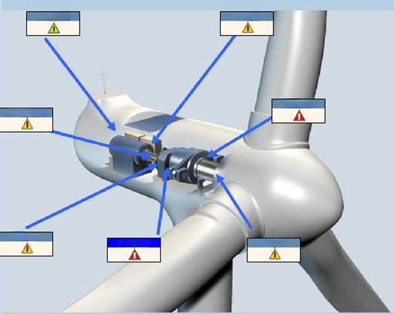
Figure 1. Vibration measurement points on the wind turbine components
Source: Original data from the work.

In each measurement point, a piezoelectric-type acceleration sensor was placed, with each sensor, in turn, recording the vibrational parameters of the component in which it was installed. In this way, it is possible to obtain the global vibration values for each measured quantity.

The measurement points are determined by means of the most important shaft bearings of the entire equipment. A wind turbine drive is defined by^[9]:

• main shaft “Main”: it is the shaft coupled to the wind turbine propellers, the wind drives the propellers which in turn rotate the main shaft;
• planetary input gear (Planet): the main shaft’s rotation is amplified thanks to a set of gears that increase the transmission ratio, so that the rotation speed of the output shaft (Shaft3) is greater than the rotation speed of the input shaft “Main”;
• intermediate shaft “Shaft2AX”: this is the intermediate shaft of the gear set, composed of pinion and crown gears, the acronym AX is used to indicate that the sensor positioning is axial in relation to the shaft.
• output shaft “Shaft3”. it is the output shaft of the speed amplifier system. This point is coupled directly to the generator, where energy is generated;
• generator coupled bearing “GEN_DE”. it is the front bearing of the generator, where the coupling with the output shaft of the speed amplification system exists;
• opposite bearing to the generator’s coupled bearing “GEN NDE”. it is the rear bearing of the generator, part of the generator shaft, where the rotor, responsible for energy generation, is installed.

The parameters measured at different points are divided between operational (which refer to the operation of the wind turbine, with “Puissance”, or generated power) and vibrational (which refer to the vibration value generated by the wind turbine at the moment of collection, such as “Ng Accélération” or Global Acceleration Level). Among the main parameters evaluated, priority was given to defining those that were statistically significant after the “stepwise” procedure for the binary logistic model^[5], and which were described below:

• “Puissance” (Power): operational parameter, obtained through the “Supervisory Control And Data Acquisition” [SCADA] system, which informs the power generated in MW/h at the time of acquisition;
• “VitesseRotation” (Rotation Speed): angular velocity of the main shaft;
• “VitesseVent” (Wind Speed): operational parameter, obtained through the SCADA system, which informs the wind speed in m/s at the time of acquisition. For the study, the highest filtered speeds from the acquisition system were considered, in order to observe the scenario of greatest vibratory effect;
• “OVL_ACC” (Global Acceleration): the global vibration level is a number obtained from a calculation that considers the various frequencies and their respective amplitudes present in the spectrum, in this case in the acceleration spectrum;
• “OVL_VEL” (Overall Vibration Velocity): the overall vibration level is a number obtained from a calculation that considers the various frequencies and their respective amplitudes present in the spectrum, in this case the Vibration Velocity spectrum. All these parameters are used by vibration analysts to identify possible failures in rotating machinery components in general.

The data referring to the measurements performed at each point were exported from the original database in .CSV format and, subsequently, loaded into the R software and RStudio IDE for processing and analysis^[10],[11].

Applying the supervised machine learning technique known as Binary Logistic Regression, the objective was to explain the probability of occurrence of the event studied, in this case, the probability of a wind turbine component entering an alarm state, as a function of the explanatory variables, which, for this study, are represented by the vibration values associated with the monitoring parameters. Therefore, the Maximum Likelihood method was applied to estimate the parameters of the logistic function; subsequently, the statistical significance of the estimated parameters was verified^[5].

Subsequently, multilevel modeling was used to capture group behaviors, as well as the random effects arising from a multilevel structure. In multilevel modeling, in addition to the nature of the data, it is important to observe the structure of the “dataset” and the arrangement of the data, so that contextual levels can be observed. Multilevel analysis then allows for the elaboration of new constructs, not observable in the logistic model.

For both situations, the metrics of greatest interest for model evaluation were the ROC curve, sensitivity, and specificity. Sensitivity refers to the percentage of correct predictions for a given criterion, considering only non-event observations, i.e., values predicted as events that truly are events. Specificity refers to the percentage of correct predictions for a given criterion, considering only non-event observations. The ROC curve, on the other hand, shows the actual behavior of the balance between sensitivity and specificity. In this sense, a given model with a large area under the ROC curve provides greater global predictive efficiency^[5].

After the Extract, Treat, and Load process, the data were submitted to logistic modeling in the R software, it was possible to extract the information that led this study. For the binary logistic analysis, the alarm STATUS of each observed parameter was considered as the response variable, which indicates the alarm levels defined in the acquisition system and that assist the vibration analyst in decision-making. Table 1 presents the types of STATUS originating from the database.

Table 1. STATUS of the parameters

CONDITION	MEANING
DNG	DANGER – Level 2 alarm
ALM	ALARM – Level 1 alarm
PRE	PRE-ALARM – Status before level 1 alarm
RAS	Absence of alarms

As for the vibration analyst, the level 2 alarm STATUS is the most critical, so at this stage the “DNG” STATUS was classified as an event occurrence, therefore it is possible with value 1 (one), and the other STATUS were classified as non-event or value 0 (zero). As can be observed in Table 2, after transforming the STATUS into binary values, the metrics regarding the quantity of events and non-events of the response variable were obtained.

Table 2. Response variable after “Dummy” process                       

Failure 0 (zero)	Success “DNG” 1 (one)
16325 (86,6%)	2525 (13,4%)

In Table 3, it is possible to observe the descriptive statistics of the most relevant explanatory variables within the “dataset”.

Table 3. Descriptive statistics of vibration parameters

Variable	Minute	1st Quartile	Median	Average	3rd Quarter	Max
Power	-0,1012	0,363	0,43	0,536	0,675	1,195
Wind Speed	0,00875	7,064	7,57	7,785	8,384	36,174
VitessRotat	0,4619	21,618	22,84	24,013	26,062	30,274
OVL_ACC	0,00660	0,2724	0,3625	0,41392	0,4810	2,2927
OVL_VEL	0,01207	0,539	0,696	0,8928	1,057	25,6592

 Subsequently, the “stepwise” procedure was applied in order to capture the greatest statistical relevance of the explanatory variables, excluding those that do not have great relevance to the model, that is, they do not present sufficient statistical significance to explain the event^[5]. Through Table 4, it can be observed that Puissance (Power) has a negative impact on the probability of failure. In this sense, it is possible to state that more powerful equipment is less subject to failures in the studied sample. It is also noted that Vitesse_Rotation (Rotation Speed) has a positive impact, that is, the higher the speed, the more subject to failures the equipment will be. Thus, other studies can be carried out with the objective of defining the ideal speed for the equipment to remain productive, but less subject to failures. Finally, the variables OVL_ACC (Global Acceleration) and OVL_VEL (Global Vibration Velocity) also presented positive coefficients, indicating a higher probability of failures with the increase of these factors.

Table 4. Estimated coefficients after “stepwise”                                                                     

Variables	Dear	Standard Error	Value	Pr (>|z|)	Sign.
(Intercept)	-11,115	1,27854	-8,693	2.00E-16	***
Power	-8,48461	0,99015	-8,569	2.00E-16	***
Rotation_Speed	0,48235	0,07591	6,354	2.1e-10	***
OVL_ACC	2,92158	0,10763	27,145	2.00E-16	***
OVL_VEL	0,8029	0,05008	19,574	2.00E-16	***

However, when analyzing the confusion matrix, which is responsible for indicating the accuracy and errors of the classification model, by confronting the actual events with the events predicted by the model, it was observed that it presents a low accuracy rate in relation to the events predicted as TRUE and that actually present a TRUE value, for a standard “cutoff” of 50%.

Table 5. Confusion matrix

		REAL
		TRUE	FALSE	Total sales (vendas)/ Invoicing (emissão de doc)
FORECAST	TRUE	233	187	420
	FALSE	2292	15429	17721
	Total sales (vendas)/ Invoicing (emissão de doc)	2525	15616	18141

Despite an interesting accuracy of around 86%, the model presented low sensitivity and high specificity, 9.2% and 98.8%, respectively, as seen in Table 6.

The area under the ROC curve is an important index for global model evaluation, as it graphically shows the relationship between specificity and sensitivity for different “cutoff” values; within this context, the model presented an area under the ROC curve of 73.9%, as can be observed in Figure 2.

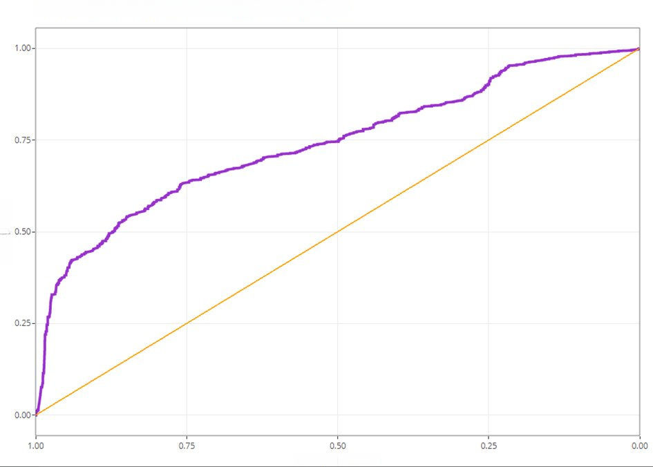
Figure 2. ROC curve
Source: Original research results.

After analyzing the results obtained by the binary logistic model, the multilevel methodology was employed to identify the random effects associated with different groups. Taking into account that the towers are distributed in various regions of the globe, the groups were separated in the “dataset”. These towers were categorized by “farms”, a term used to designate wind farms. It is worth noting that a single region can house multiple “farms”.

The research analyzed a total of 117 wind turbines. These turbines are distributed in parks containing up to 11 turbines each and are located on three distinct continents: Asia, Europe, and North America. It is worth noting that a single geographical region can house several “farms”. For example, in Europe, there are the “farms” WF1, WF2_L1, and WF2_L2, as illustrated in Figure 3.

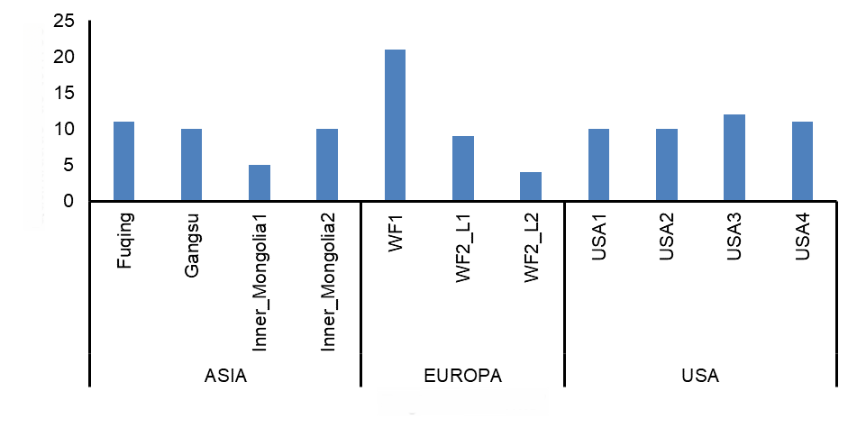
Figure 3. Number of towers per “farms” and region
Source: Original research results

Since multilevel hierarchical models are capable of capturing the decomposition of variance of random group effects, where the response variable is categorical, as observed so far, the principle was precisely to dichotomize the STATUS variable, in an analogous way to what had been done in the analysis with the binary logistic methodology[5]. However, this time, in addition to considering the category “DNG” (Danger) as an event, the category “ALM” (Alarm) was also included as an event. Table 7 shows how the counts of non-events x events turned out after dichotomizing the STATUS variable. It is noted that, in relation to the first model, the increase in the number of events was approximately 265%, thus resulting in 63.10% of non-events and 36.9% of events.

Table 7. Response variable after “Dummy” process                                                  

Failure 0 (zero)	Success “DNG” and “ALM” 1 (one)
11447 (63,10%)	6694 (36,9%)

Still in the transformation of the “dataset”, the derivation of the MEASUREMENT DATE variable into “dummies” was included, with the objective of observing the influence of climatic effects (seasons of the year) on the response variable. Thus, the months were arranged as categories for the creation of the “dummies”. After this procedure, the multilevel model was generated, which presented the following parameters after estimation, according to Table 8.

Table 8. Results of the multilevel model with random intercepts

Variables	Dear	Standard Error	value	Pr(>|z|)	Signature
(Intercept)	-2,15826	0,66310	-3,25	0,00113	**
Power	-3,63266	0,13518	-26,87	< 2e-16	***
OVL_ACC	7,00496	0,15169	46,18	< 2e-16	***
OVL_VEL	1,81259	0,05710	31,74	< 2e-16	***
Arret_Acceleration	-0,71068	0,04476	-15,88	< 2e-16	***
month_2	0,73728	0,06296	11,71	< 2e-16	***
month_3	0,18792	0,06620	2,84	0,00453	**
month_4	0,29344	0,06575	4,46	8.08e-06	***
month_5	-0,18472	0,06084	-3,04	0,00240	**
month_7	0,17836	0,05842	3,05	0,00227	**
month_8	0,16693	0,05680	2,94	0,00330	**
month_9	-1,15504	0,12609	-9,16	< 2e-16	***
month_10	0,23240	0,11799	1,97	0,04889	*
month_11	-2,16955	0,12854	-16,88	< 2e-16	***
month_12	-0,68953	0,10325	-6,68	2.41e-11	***

From Table 8, it is possible to perceive that the signs of the coefficients remained compatible with the multilevel logistic regression, however, with different values. The different values were due to other variables that were inserted into the fixed effects, especially the months, as well as the random effects region and “farm”. As the months were inserted as “dummies”, their results are in comparison to January (mes_1), which was inserted as the reference variable. In this way, it can be interpreted that November (mês_11) has a lower probability of failure in relation to January; on the other hand, February has a higher probability in relation to January. The parameters of the random effects were also estimated, as presented in Table 9.

Table 9. Statistics of the effects

Group Names		Variance	Standard deviation
region	(Intercept)	0,04424	0,2103
agricultural property	(Intercept)	4,32420	2,0795

Table 9 shows that the greater variance occurs between different farms and that the variance between regions is discrete. To evaluate the confusion matrix, a graph was created in R software, aiming to identify the optimal intersection point between sensitivity and specificity values. As illustrated in Figure 4, the cutoff point selected for the construction of the confusion matrix was set at 30%.

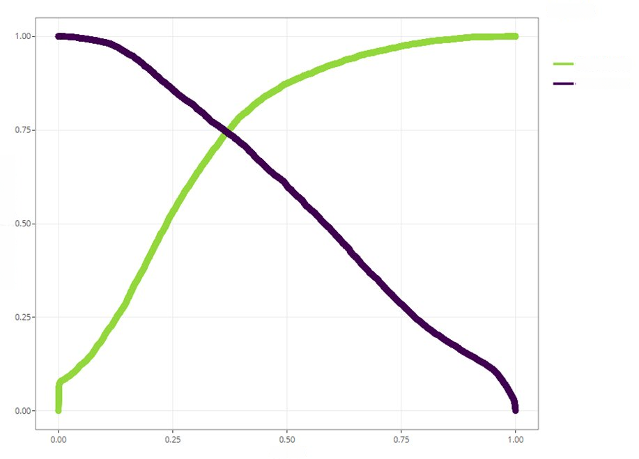
Figure 4. Sensitivity x specificity graph
Source: Original research results

With the best “cutoff” defined, it was then possible to generate the confusion matrix and the parameters for model evaluation, such as sensitivity values, i.e., how accurate the model is in classifying events, and specificity, i.e., how accurate the model is in avoiding false positives. A considerable increase in sensitivity compared to the binary logistic model is noteworthy (about 71.8% increase), while specificity showed a slight decrease. Table 10 shows the confusion matrix and evaluation parameters.

Table 10. Confusion matrix

		REAL
		TRUE	FALSE	Total sales (vendas)/ Invoicing (emissão de doc)
FORECAST	TRUE	6799	4922	11721
	FALSE	1585	8317	9902
	Total sales (vendas)/ Invoicing (emissão de doc)	8384	13239	21623

Table 11. Evaluation parameters

Metric	Value
Accuracy	0,6991
Sensitivity	0,8109
Specificity	0,6282
Balanced accuracy	0,7196

When analyzing Table 11 in comparison with Table 6, it is evident that some metrics showed a decline, while others demonstrated improvements. This change is due to the point at which the cutoff was applied. In the case of the multilevel logistic model, a cutoff of 30% was chosen, in contrast to the binary logistic model, in which the standard cutoff of 50% was used. However, it is crucial to highlight that the objective of adjusting the “cutoff” value was achieved, meaning that the metrics values were successfully balanced, but it is worth noting that the ideal “cutoff” point may vary depending on the phenomenon under study.

In addition to the metrics evaluated above, another important metric is the area under the ROC curve, as it plays a crucial role in the comprehensive evaluation of the model. In this context, it is noteworthy that the multilevel logistic model achieved an area under the ROC curve of 81.9%, representing an increase of 8% compared to the binary logistic model, as illustrated in Figure 5.

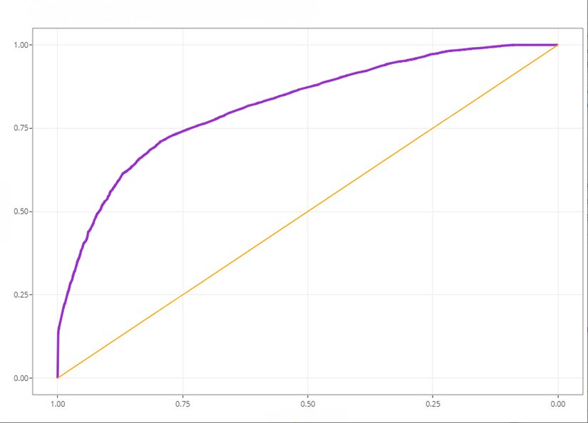
Figure 5. ROC curve
Source: Original research results

The study was successful in achieving its main objective by demonstrating the respective ROC curves of the binary logistic and multilevel logistic models, so it was possible to observe that the latter presents greater global predictive efficiency; thus, the application of multilevel modeling, taking into account the influence of random effects that cannot be captured with binary logistic modeling, proves to be a relevant technique for predicting failures in wind turbines.

References

[1] Brito J. N. 2017. Plano De Manutenção de Ativos Físicos Como Parte Estratégica do Negócio. In: XVII Congresso Nacional de engenharia mecânica e industrial, 2017, Joinville, SC, Brasil. Disponível em: <http://doi.org/10.17648/conemi-2018-91231>. Acesso em: 16 out. 2022.

[2] Brito J. N. Marques A. C. 2019. Importância da manutenção preditiva para diminuir o custo em manutenção e aumentar a vida útil dos equipamentos. Brazilian Journal of Development. 5(7): 8913-8923. Disponível em: <https://doi.org/10.34117/bjdv5n7-095>. Acesso em: 16 out. 2022

[3] Hashemian H. M. 2011. State-of-the-Art Predictive Maintenance Techniques. IEEE Transactions on Instrumentation and Measurement. 60(1): 226–236. Disponível em: < https://doi.org/10.1109/TIM.2009.2036347>. Acesso em: 28 set. 2022.

[4] Carvalho T. P., et al. 2019. A systematic literature review of machine learning methods applied to predictive maintenance. Computers & Industrial Engineering. 137: 106024. Disponível em: <https://doi.org/10.1016/j.cie.2019.106024>. Acesso em: 12 out. 2022.

[5] Fávero L. P.; Belfiore, P. 2017. Manual de análise de dados: estatística e modelagem multivariada com Excel®, SPSS® e Stata®. Elsevier, Rio de Janeiro, Brasil.

[6] Confortini, D; Fávero L. P. 2010. Modelos multinível de coeficientes aleatórios e os efeitos firma, setor e tempo no mercado acionário Brasileiro. Pesquisa Operacional. 30(3): 703-727. Disponível em: <https://doi.org/10.1590/S0101-74382010000300011>. Acesso em: 12 out. 2022.

[7] Al-Musthafa M. I. Learning Vector Quantization Based Vibration Analysis for Steam Power Plant Rotating Equipment Fault Diagnosis. In: 2019 International Conference on Technologies and Policies in Electric Power & Energy. IEEE, 2019. p. 1-3. Disponível em: < https://dx.doi.org/10.1109/IEEECONF48524.2019.9102521>. Acesso em: 10 out. 2022.

[8] Soto-Ocampo, C. R.; Mera J. M.; Cano-Moreno J. D.; Bernardo J. L. G. Low-cost, high-frequency, data acquisition system for condition monitoring of rotating machinery through vibration analysis-case study. Sensors, v. 20, n. 12, p. 3493, 2020. Disponível em: <https://dx.doi.org/10.3390/s20123493>. Acesso em: 16 out. 2022

[9] Manwell J. F.; Mcgowan, Jon G.; Rogers, Anthony L. Wind energy explained: theory, design and application. John Wiley & Sons, 2010. Disponível em: <http://doi.org/10.1002/9781119994367>. Acesso em: 16 out. 2022.

[10] R Core Team. R: A language and environment for statistical computing. Viena, Áustria: R Foundation for Statistical Computing, 2022. Disponível em: <https://www.R-project.org/>. Acesso em: 10 set. 2022.

[11] RStudio Team. RStudio: Integrated Development Environment for R. Boston, MA: RStudio, PBC, 2022. Disponível em: <https://www.rstudio.com/>. Acesso em: 10 set. 2022.

How to cite

Silva J. G. M.; Silva J. E. The use of the multilevel approach for predicting failures in wind turbines. E&S Journal. 2023; 4: e20230110.

About the authors

João Gilberto Máximo Da Silva , Avenue João Galego, 988 – Santa Maria; 09560-340 – São Caetano do Sul, São Paulo, Brazil.

José Erasmo Silva , Advisor Professor MBA Data Science and Analytics, Rua Maria Társia, 51 – Jardim Elite; 13417-440. Piracicaba, São Paulo, Brazil.

Download link: PDF