Optimization of tax audit actions through company ranking using machine learning

Junior, Autores: Giovana Amorim Zanato e Cláudio Tucci

doi:10.22167/2675-6528-2024082E

Article

Technology

October 23, 2025

Optimization of tax audit actions through company ranking using machine learning

^{Authors: Giovana Amorim Zanato and Cláudio Tucci Junior}

^{DOI: 10.22167/2675-6528-2024082
E&S 2025, 6: e2024082}

Tax audit is a central element of tax collection and compliance in the public sector, it ensures the correct application of norms and plays a strategic role in enabling public policies through the collected revenue^[1]. With the transition from the Tax on Circulation of Goods and Services (ICMS) to the Tax on Goods and Services (IBS)^[2], scheduled for 2026, the relevance of data science and machine learning methods as tools to identify tax evasion risks grows, they provide cost reduction, greater transparency and detection of outliers when comparing the behavior of a taxpayer with that of their reference population^[3].

Previous studies on the use of machine learning in tax auditing have demonstrated its effectiveness in detecting tax fraud. Ruzgas and Kizauskiene^[4] developed a study with several models for detecting tax crimes and showed that the data mining technique identifies tax evasion and extracts hidden knowledge applicable to reducing revenue losses from evasion.

Silva and Rigitano^[5] conducted a case study of financial fraud with Bayesian networks on data from taxpayers in São Paulo, Brazil. Wahab and Bakar^[6] applied a set of machine learning algorithms to classify income tax at the Inland Revenue Board of Malaysia and verified the effectiveness of different machine learning algorithms in audit selection. Shi and Dong^[7] studied a heterogeneous graph neural network model to support tax evasion detection. These works highlight the potential of machine learning to improve the accuracy and efficiency of tax audits.

The report by the Organisation for Economic Co-operation and Development (OECD) (Tax audits in a changing environment) emphasizes that tax audits should be designed as instruments of tax compliance and risk-based monitoring, capable of identifying potential non-compliance preventively, reinforcing voluntary compliance with tax obligations, and strengthening the legitimacy and transparency of the tax system^[8].

In this context, this study uses property data from the Goiás State Secretariat of Economy, with historical records of audits and information declared by taxpayers to compare different machine learning techniques with the objective of classifying companies with a higher risk of tax non-compliance regarding ICMS.

Therefore, this study aims to apply and compare machine learning models to rank companies, in order to more effectively direct fiscal audit actions, reduce costs, increase transparency, and strengthen the fight against unfair competition.

This research adopts a quantitative approach, based on numerical data from tax declarations and audit records, subjected to statistical and machine learning techniques, and has a descriptive character by analyzing taxpayer behavior patterns and comparing the performance of different predictive models to prioritize fiscal audit actions^[9].

According to Alpaydin^[10], machine learning is the area of artificial intelligence that develops methods for computers to identify patterns from data and make predictions without explicit programming. A machine learning model is the mathematical representation built from data, capable of identifying patterns and generating predictions or classifications in new situations^[11].

The target variable, which represents the outcome the model seeks to predict, is quantitative and indicates the financial value, in reais, calculated from tax audits conducted by tax auditors from the Goiás State Secretariat of Economy, between 2019 and 2023, for 448 medium and large retail companies. This variable, named TRIBUTAVEL_AUTO in the database used, represents the amount of ICMS evaded by the taxpayer in the analyzed fiscal year (Table 1) which represents the value that the model in question intends to predict for those taxpayers not yet audited.

^{Table 1. Traffic violation data¹}

^{Variable name}	^Description
^{Taxable event period}	^{Month and year referring to the assessed generating event}
^Taxable_auto	^{Nominal value of the levied Tax on Circulation of Goods and Services (ICMS)}

^{Source: Original survey data.
Note. ¹The infringement notice is the formal document that initiates the administrative tax process.}

The explanatory variables serve as parameters to estimate the probable value of evaded ICMS. The selection of explanatory variables considered theoretical criteria and practical relevance for ICMS calculation, prioritizing information directly related to taxpayers’ fiscal behavior and sectoral specificities. Redundant or highly correlated variables, such as “collected ICMS,” were avoided to reduce multicollinearity and preserve model interpretability. However, the possibility of selection bias arising from the database itself, which reflects only taxpayers with complete and consistent EFDs, is acknowledged. To mitigate this risk, integrity and coherence checks of the information used were adopted.

The taxpayer’s calculation, represented in record E110 of the Digital Tax Bookkeeping (EFD)^[12,13], consolidates all of the taxpayer’s monthly fiscal activity, and as detailed in Table 2, constant variables were selected in this record during the audited periods.

Table 2. Monthly taxpayer’s calculation reported in the Digital Tax Ledger (EFD)

^{Variable name}	^{Field in EFD}	^Description
^Debit	^{VL_TOT_DEBITOS}	^{Total value of debits for outflows and services with tax debit}
^{Debit_adjustment_document}	^{VL_AJ_DEBITOS}	^{Total value of debit adjustments arising from fiscal document}
^{Debit_adjustment}	^{VL_TOT_AJ_DEBITOS}	^{Total debit adjustment value}
^{Credit_reversal}	^{CREDIT_REVERSAL_VALUE}	^{Total value of credit chargebacks}
^Credit	^{Total Credits Value}	^{Total value of credits for entries and acquisitions with tax credit}
^{Credit_adjustment_document}	^{VL_TOT_AJ_CREDITOS}	^{Total value of credit adjustments arising from fiscal document}
^{Credit_adjustment}	^{VL_AJ_CREDITOS}	^{Total value of credit adjustments}
^{Debit_Reversal}	^{DEBIT_REVERSAL_VALUE}	^{Total value of debit chargebacks}
^{Credit_balance_previous}	^{VL_SLD_CREDOR_ANT}	^{Credit balance from the previous period transferred to the reference period}
^Net_balance	^{Spatially lagged variable}	^{Outstanding balance}
^Deduction	^VL_TOT_DED	^{Total value of deductions}
^{ICMS payable}	^{VL_ICMS_RECOLHER}	^{Total value of the Tax on Circulation of Goods and Services (ICMS) to be paid to the public coffers}
^{Credit_balance_t}	^{VALUE_CREDITOR_BALANCE_TO_TRANSFER}	^{Total value of the credit balance that, when existing, will be carried over to the next period}
^Extra_output	^DEB_ESP	^{Collected or to be collected values, extra-calculation}

^{Source: Original survey data.
Note. Data from record E110, block E, of the Digital Tax Ledger (EFD)[13].}

The tax burden of the sector in which the company operates (Table 3) also comprises the set of explanatory variables, as it brings fiscal particularities of each retail sector, significantly impacting the model’s outcome.

Table 3. Tax burden of the sector

^{Variable name}	^Description
^Ct_sector	^{Tax burden of the sector, calculated by selecting invoices for outgoing operations by type of commercial activity and by dividing the sum of the value of the Tax on Circulation of Goods and Services (ICMS) by the sum of the nominal values of the products}

^{Source: Original survey data.
Note: Data from constant output operations in record C190 of the Digital Fiscal Record (EFD) [13] were used.}

All the necessary data for the work are stored in the databases of the Secretariat of Economy of the State of Goiás. The extraction, selection, and cleaning of the data were performed with the SAS Enterprise Guide v.9.2 (Statistical Analysis System, Cary, NC, USA) software, through the creation of flows for generating output files in CSV format.

The development of the algorithms occurred in the R program, with the tidyverse, rgl, jtools, Rmisc, caret, neuralnet libraries applied in the processing and analysis of the data. The data worked with do not present contributor identification and the values are itemized to make identification impossible, in line with specific fiscal secrecy regulations.

In the case under study, companies with fiscal compliance were not included due to the impossibility of determination, as a company selected for audit presents some indication of irregularity. On the other hand, it is not possible to state that the companies not selected for audit are in full fiscal regularity regarding ICMS assessment.

Among the available machine learning techniques, multivariate linear regression models, random forest, and artificial neural networks were selected for comparative study. The model that presents the best performance, according to the specific evaluation metrics, will be applied to the database of the other contributors, with the aim of estimating the potential value of omitted ICMS from the provided variables and supporting the prioritization of inspection actions.

The study was initiated with the development of the multivariate linear regression technique in order to understand the behavior of the phenomenon in question from the explanatory variables. With the historical data from tax audit results, it was expected that the model would provide an estimate of the levied ICMS, that is, the amount of ICMS omitted and not collected by state public coffers, according to the monthly calculation and the tax burden of the analyzed taxpayer’s sector.

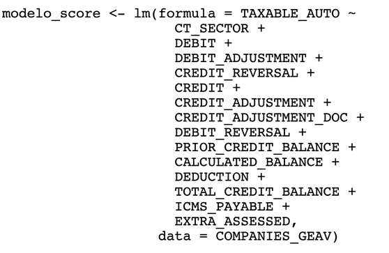
The normalization of variables and the initial execution of the model, through the lm command (Figure 1), revealed the presence of parameters without statistical significance, which indicated the need for refinement. To include only variables with statistically significant influence on the outcome in the final model, the stepwise^[14] procedure was applied, which gradually evaluates and removes variables without relevant contribution.

^{Figure 1. Initial multivariate linear regression algorithm, before the Box-Cox procedure
Source: Original research data.}

Next, the Box-Cox transformation^[15] was applied, a mathematical technique that adjusts variables to approximate their distribution to normality, which strengthens the validity and reliability of the model. The results are described in Table 4.

Table 4. Result of the model estimation after Box-Cox transformation and stepwise procedure

^{Variable Name}	^Dear	^Standard	^Error	^t-statistic	^{Select (or mark)}
^{(Interception)}	^0,05591	^0,01297	^4,312	^2e-05	^***
^CT_SECTOR	^-0,05005	^0,02213	^-2,262	^0,02419	^*
^DEBIT	^-4,18415	^1,86388	^-2,245	^0,02528	^*
^{DEBIT_ADJUSTMENT}	^-0,19378	^0,08748	^-2,215	^0,02727	^*
^{CREDIT_REVERSAL}	^-0,13765	^0,05635	^-2,443	^0,01498	^*
^CREDIT	^2,65803	^1,13202	^2,348	^0,01932	^*
^{CREDIT_ADJUSTMENT}	^0,79261	^0,29350	^2,701	^0,00719	^**
^{DEBIT_REVERSAL}	^1,02801	^0,07873	^13,057	^<2e-16	^***
^{CALCULATED_BALANCE}	^0,94823	^0,45529	^2,083	^0,03787	^*
^DEDUCTION	^0,12780	^0,05925	^2,157	^0,03155	^*
^EXTRA_APUR	^-0,21454	^0,06758	^-3,175	^0,00161	^**

Source: Original survey data.
Note. Standard residual error: 0.07244 on 434 degrees of freedom; R-squared: 0.437; Adjusted R-squared: 0.424; F-statistic: 33.69 on 10 and 434 DF; p-value: < 2,2e-16; Pr(>t): significance levels: ***: between 0 and 0.001; **: between 0.001 and 0.01; *: between 0.01 and 0.05.

After generating the model, the Shapiro-Francia test was applied, a simple and robust test for
checking residuals for normality. As presented in Table 5, the model under study showed P-value = 2.2e-16, which indicates incompatibility with a normal distribution, and the model was not suitable for the study in question^[14].

^{Table 5. Shapiro-Francia normality test}

^{data: step_model_bc_SCORE$residuals}

^{W = 0.51394, p-value < 2.2e-16}

^{Source: Original survey data.}

After the initial analysis, it was found that the linear regression model was not suitable for the study, as the data presented characteristics of non-linearity. Therefore, the random forest, a machine learning algorithm recognized for its robustness, was selected. This technique combines the power of multiple decision trees and is effective in handling complex and non-linear relationships in the data. In addition to increasing model accuracy, the approach minimizes the risk of overfitting (excessive fitting to the data) and ensures that the conclusions are more reliable and generalizable to other scenarios^[16].

The first step in applying the technique, after loading the data, is to split the dataset into training, validation, and testing sets. The training set is used to adjust the model’s parameters and for it to learn patterns from the data. Regarding the validation set, it is used during training to define hyperparameters, compare models, and avoid overfitting. And the test set is applied only after training and validation; it provides an independent way to measure the model’s performance on unseen data, which allows evaluating its generalization capability. In the model under study, the training set comprised 60% of the data, the validation set 20%, and the test set the remaining 20%.

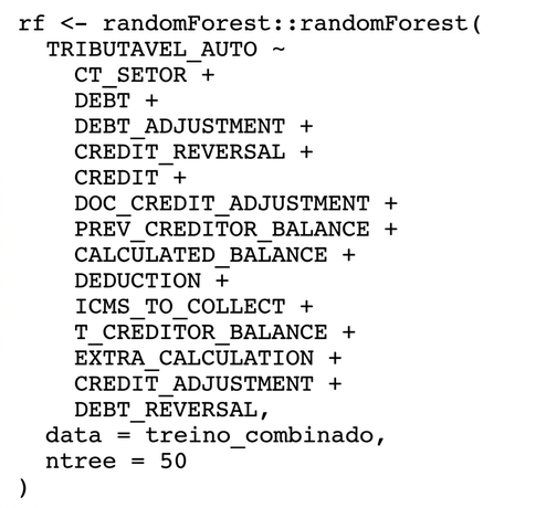
Several combinations of variables and parameter settings were tested. The best results occurred when the AJ_DEBITO_DOC variable was disregarded, as it proved to be irrelevant to the model. The parameter setting that presented the highest R² (proportion of the variability of the target variable explained by the model) on the test set used the validation set incorporated into the training set, in order to expand the training set.

The model was trained with 50 trees (ntree = 50), as represented by the algorithm in Figure 2.

^{Figure 2. Algorithm ofrandom forest
Source: Original research data.}

The R² obtained on the test set was 61%, with a mean squared error (Mean of Squared Error – MSE) = 2.496516e+14 and an explained variability percentage of 15.12%, as presented in Tables 6 and 7.

_{Table 6. Model evaluation using the random forest technique}

^Basis	^MSE¹	^R2²
^Training	^5.816345e+13	^0,8022467
^Test	^2.239706e+14	^0,6133123

^{Source: Original survey data.
Note: ¹MSE: Mean Squared Error – mean squared error. ²R^²: coefficient of determination.}

_{Table 7. Characteristics of the variable created with the random forest algorithm}

^{Type of random forest}	^Regression
^{Number of trees}	⁵⁰
^{Number of variables tested at each split}	⁴
^{Mean squared residuals}	^2.496516e+14
^{Percentage of variable explainability (%)}	^15,12

Source: Original survey data.

The analysis of the variables in the test base, in light of the specific context of the problem, indicates that the R² of 61% can be considered moderately good, that is, 61% of the variability of the TRIBUTAVEL_AUTO variable is explained by the model. However, upon observing an explainability percentage of variables of 15, 12 and an MSE of 2.239706e+14, it is concluded that the model does not present adequate predictive capacity and may not constitute a satisfactory solution for the problem. From this evaluation, the need to analyze the problem with the artificial neural network technique was identified.

Artificial neural networks were inspired by the functioning of the human brain. These computational systems are composed of interconnected units, called artificial neurons, which process information and learn complex patterns from data. The structure of neural networks consists of layers of neurons, in which each neuron performs mathematical operations to transform input data into useful outputs. The main characteristic of neural networks is their learning ability, with constant improvement of the model’s performance, whose training occurs through an iterative process of adjusting the weights between nodes, using techniques such as gradient descent.^[17]

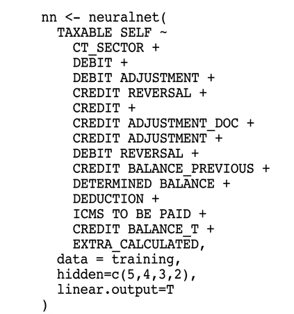
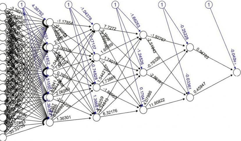
The first step in applying the neural network model to the case study consisted of normalizing the variables, followed by dividing the database into 70% for training and 30% for testing. The next step was the execution of the neural network algorithm, demonstrated in Figure 3. Several combinations of explanatory variables and hyperparameters were tested. As in the random forest model, the best results occurred when the AJ_DEBITO_DOC variable was disregarded, as it proved to be irrelevant to the model. The combination of hyperparameters that presented the best performance includes four intermediate layers: the first with five neurons, the second with four, the third with three, and the fourth with two, according to the model architecture presented in Figure 4, and the use of an activation function at the output.

^{Figure 3. Neural network algorithm
Source: Original research data.}

^{Figure 4. Graphical representation of the neural network model architecture for the case under study with the layers, nodes, and respective weights
Source: Original research data.}

The model presented an MSE of 0.007816 on the test set, as shown in Table 8. It
provides a measure of the overall accuracy of the neural network model with respect to the test data. The lower the MSE value, the closer the predictions are to the Actual Values^[11]. Since the MSE was calculated on independent test data, the model demonstrates good generalization capability, which allows its application to other bases of retail contributors and the identification of those with potential indications of tax evasion.

Table 8. Model evaluation data using the neural network technique

^Basis	^MSE¹	^{^R2²}
^Training	^0,002264842	^0,704415
^Test	^0,007816353	^0,3610342

Source: Original survey data.
Note: Note: ¹MSE: Mean Squared Error – mean squared error. ²R²: coefficient of determination.

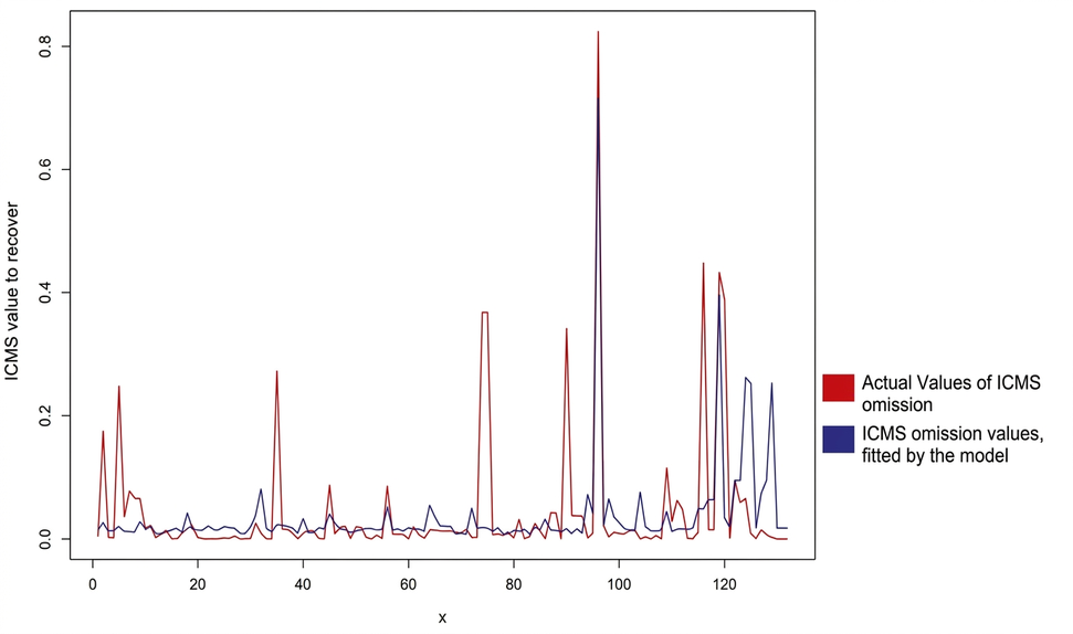
The graph presented in Figure 5 was generated from the artificial neural network model and shows,
in red, the actual values of ICMS omission, i.e., the values of ICMS assessed in tax actions, and, in blue, the values of omitted ICMS predicted by the model in the test base.

^{Figure 5. Graphical representation of the neural network model for the case under study
Source: Original research data.
Note. Graph generated in R software from the model generated in the same software.}

The results of this study corroborate the findings of previous research, which indicate that neural network models are effective in detecting complex and non-linear patterns in fiscal data^[18]. Although the random forest model presented a superior R², the neural network’s low MSE highlights its ability to provide more accurate predictions.

The methodological approach of this study — which combined multivariate linear regression, random forest, and neural networks — contributed not only to evaluating different levels of statistical complexity but also to generating practical interpretations relevant to fiscal management. Understanding the relationships between variables allowed for the identification of patterns associated with the probability of tax evasion, providing subsidies for more efficient targeting of audits and for the more rational use of enforcement resources.

The comparison between the models also evidenced the potential of machine learning techniques in increasing prediction accuracy, which can result in reduced operational costs and a positive impact on revenue collection, by concentrating efforts on taxpayers with higher fiscal risk. Thus, the results obtained extrapolate the methodological field and offer concrete decision support tools in tax administration.

The in-depth analysis of ICMS and the identification of tax evasion patterns offer important subsidies for the future management of IBS, as both share structural characteristics: they essentially impact the circulation of goods and services, are indirect taxes whose burden is transferred to the final consumer, and adopt non-cumulativeness, with tax credits for the tax paid in previous stages of the chain. However, IBS presents a significant advantage regarding the breadth of its incidence base, which will cover not only operations currently subject to ICMS, but also other services, rentals, and financial activities^[2].

Furthermore, its regulation will be more uniform, unlike ICMS, whose normative discipline is fragmented among the states. In this scenario, the available datasets for fiscal analyses tend to be substantially larger and more consistent. This factor favors the application of machine learning models with less susceptibility to noise and greater capacity for robust identification of complex relationships.

The study fulfilled its objective of investigating how artificial intelligence models, specifically neural networks, can be applied to identify tax evasion patterns and provide subsidies for tax management. Despite some limitations, such as the restriction to 15 specific variables and the dependence on data from selected sectors, which, at the state level, specifically in the State of Goiás, constitute a restricted population for the study and may even be a limitation to the generalization of the results, it was possible to develop a model with a high level of predictability for the observed values.

By identifying complex evasion patterns, the proposed model can be adapted to the new Brazilian tax system, in order to assist in the development of more robust auditing and compliance mechanisms. Future research can explore broader databases, include additional variables, and evaluate the model’s application in different sectors, with the aim of improving the accuracy and effectiveness of enforcement strategies in the context of tax reform.

REFERENCES

^{[1] Santos, C. 2015. Auditoria Fiscal e Tributária. 3ed. São Paulo, SP: IOB.}

^{[2] Brasil. 1988. Constituição da República Federativa do Brasil. Brasília, DF: emenda constitucional n. 132. Disponível em: http://www.planalto.gov.br/ccivil_03/constituicao/constituicao.htm . Acesso em: 15 set. 2025}

^{[3] Alexopoulos, A.; Kotsogiannis, C.; Dellaportas, P.; Olhede, S. C.; Gyoshev, S.; Pavkov, T. 2025. A network approach to detect Value Added Tax fraud. Department of Economics, AUEB, Greece. Disponível em: https://arxiv.org/pdf/2106.14005 . Acesso em: 15 set. 2025.}

^{[4] Ruzgas, T.; Kižauskienė, L.; Lukauskas, M.; Sinkevičius, E.; Frolovaitė, M.; Arnastauskaite, J. 2023. Tax Fraud Reduction Using Analytics in an East European Country. MDPI (Multidisciplinary Digital Publishing Institute). Disponível em: https://www.mdpi.com/2075-1680/12/3/288 . Acesso em: 15 set. 2025.}

^{[5] Silva, L. S.; Rigitano, H. C.; Carvalho, R. N.; Souza, J. C. F. 2016. Bayesian Networks on Income Tax Audit Selection – A Case Study of Brazilian Tax Administration. Brasília, DF. Disponível em: https://ceur-ws.org/Vol-1663/bmaw2016_paper_3.pdf . Acesso em: 15 set. 2025.}

^{[6] Wahab, R. A. S. R.; Bakar, A. A. 2021. Digital Economy Tax Compliance Model in Malaysia using Machine Learning Approach. Disponível em: https://www.ukm.my/jsm/pdf_files/SM-PDF-50-7-2021/20.pdf . Acesso em: 15 set. 2025.}

^{[7] Shi, B.; Dong, B. 2023. An edge feature aware heterogeneous graph neural network model to tax evasion detection. Artigo. Expert System with Applications: An International Journal. Disponível em: https://dl.acm.org/doi/10.1016/j.eswa.2022.118903 . Acesso em: 15 set. 2025.}

^{[8] Organização para a Cooperação e Desenvolvimento Econômico (OECD). 2017.. Tax Changing Tax Compliance Enviroment and the Role of Audit. 2017 OCDE – Organização para a Cooperação e Desenvolvimento Econômico. Paris. Disponível em: https://www.oecd.org/en/publications/the-changing-tax-compliance-environment-and-the-role-of-audit_9789264282186-en.html . Acesso em: 15 set. 2025.}

^{[9] Creswell, J. W. 2022 Research design: qualitative, quantitative, and mixed methods approaches. 6ed. Thousand Oaks, CA, EUA: Sage.}

^{[10] Alpaydin, E. 2020. Introduction to Machine Learning. 4ed. Cambridge, MA, USA: The MIT Press.}

^{[11] Hastie, T.; Tibshirani, R.; Friedman, J. 2009. The Elements of Statistical Learning: Data Mining, Inference, and Prediction. 2ed. New York: Springer.}

^{[12] Brasil. 2007. Decreto n. 6.022, de 22 de janeiro de 2007. Institui o Sistema Público de Escrituração Digital – Sped. Receita Federal do Brasil, Brasília, DF. Disponível em: http://www.planalto.gov.br/ccivil_03/_ato2007-2010/2007/Decreto/D6022.htm. Acesso em: 15 set. 2025.}

^{[13] Sistema Público de Escrituração Digital.2023. Guia prático da escrituração fiscal digital – EFD ICMS/IPI. v.3.1.5. Disponível em: http://sped.rfb.gov.br/arquivo/show/7273. Acesso em: 15 set. 2025.}

^{[14] Fávero, L. P.; Belfiore, P. 2022. Análise de dados: estatística e modelagem multivariada com Excel, SPSS e Stata. Rio de Janeiro: LTC.}

^{[15] Box, G. E. P.; Cox, D. R. 1964. An Analysis of Transformations.Journal of the Royal Statistical Society. Series B. 26(2). 211-252.}

^{[16] Angshuman, P.; Dipti, P. M.; Prasun, D.; Abhinandan, G.; Appa, R. C.; Saurabh, K. 2018. Random Forest aprimorado para classificação. IEEE Transactions on Image Processing, 27. Disponível em: https://ieeexplore.ieee.org/document/8357563 . Acesso em: 15 set. 2025.}

^{[17] Hardesty, L. 2017. Explained: Neural networks: Ballyhooed artificial-inteligence technique known as “deep learming” revives 70-years-old idea. MIT News. Disponível em: https://news.mit.edu/2017/explained-neural-networks-deep-learning-0414. Acesso em: 15 set. 2025.}

^{[18] Pérez López, C.; Delgado Rodríguez, M.J.; Lucas Santos, S. 2019. Tax Fraud Detection through Neural Networks: An Application Using a Sample of Personal Income Taxpayers. Future Internet. 11(4), p. 86. doi:10.3390/fi11040086. Disponível em: https://www.mdpi.com/1999-5903/11/4/86 . Acesso em: 15 set. 2025.}

COMO CITAR

^{Zanato, G.A.; Tucci Jr, C. Otimização das ações de auditoria fiscal através do ranqueamento de empresas utilizando aprendizado de máquina. Revista E&S. 2025; 6: e2024082.}

ABOUT THE AUTHORS

^{Giovana Amorim Zanato – Specialist in Data Science and Analytics. Tax Auditor of the State Revenue. Secretariat of Economy of the State of Goiás. Avenida Vereador José Monteiro, 2233, Setor Vila Nova, 74653-900, Goiânia, Goias, Brazil.}

^{[/3]Doctor of Social Sciences. Supervising Professor. Avenida Paulista, 1159, Suites 612 and 613, Cerqueira César, São Paulo, SP, Brazil.}