
Technology
September 11, 2025
The covid-19 pandemic and the demand for air passenger transport on domestic flights
Authors: Laís Kimie Oshiro Caldeira and José Erasmo Silva
DOI: 10.22167/2675-6528-2023111
E&S 2025, 6: e2023111
The ability to predict the demand for a given service is a critical activity, yet it represents a challenge for managers in different industries. In the airline sector, demand forecasting impacts short-to-long-term planning, encompassing decisions about airport expansion or the construction of new ones, the planning of airlines, airport operators, and aircraft manufacturers, as well as the activities of other agents integrated into this complex supply chain[1].
The covid-19 pandemic, declared in 2020, unexpectedly affected the entire sector and frustrated any demand forecast projected for the subsequent months. According to the National Civil Aviation Agency (Anac)[2], in August 2021 – more than a year after the pandemic declaration – the number of passengers transported on domestic flights was still 30% lower than that recorded in August 2019.
Given this scenario, it becomes necessary to understand how demand reacted to the reduction of sanitary measures, the advancement of vaccination, and the recovery of other economic sectors. Thus, this study aims to identify a model capable of explaining the demand for air transport in the domestic market as a result of these factors, which provides a reference for future similar situations that impact the sector.
The first stage of this study consisted of data collection and processing. Public databases were used for the period from January 2020 to January 2022. Data from periods prior to 2020 were included solely for the purpose of discussing the results.
The dependent variable, which represents the phenomenon under study, is the demand for air passenger transport in the domestic market. The database used was extracted from the statistical data of air transport in Brazil, published by ANAC[3], which provides detailed information about the sector. To reflect the demand, the variable “paid passengers” was selected, filtering only information related to domestic flights, whether regular or non-regular.
Data of different natures were used as independent (or explanatory) variables. These variables are so named because they are used to explain the variations observed in the dependent variable. Information related to the pandemic, such as the number of daily new cases of covid-19, was extracted from the Ministry of Health’s coronavirus dashboard[4]. Records of vaccination against covid-19 in Brazil were obtained from the Coronavirus Pandemic[5] database with information regarding the percentage of vaccinated people, fully vaccinated people, and those who received the booster dose.
The airfare was also considered, extracted from the microdata of commercialized airfares, published by ANAC[6]. The monthly average fare was used, calculated from the weighted average between the prices charged and the number of tickets sold. Furthermore, data on the price of aviation fuel were incorporated, used as an instrumental variable for the value of tickets, extracted from the aviation fuel price table provided by Petrobras[7], from which the national average was obtained.
Finally, data regarding employment level and Gross Domestic Product (GDP) were extracted from the Ipeadata portal, including the “Labor force participation rate”[8] – which corresponds to the percentage of people in the labor force in relation to the working-age population – and the monthly GDP records[9]. Table 1 presents a summary of the final database used. All records were organized with monthly periodicity.
Table 1. Database summary
| Variable | Average | Maximum | Minimum | Standard deviation |
| domestic_passengers | 4.612.943 | 9.304.796 | 399.557 | 2.401.210 |
| vaccinated_people | 23,03% | 79,59% | 0,0% | 31,62 |
| fully_vaccinated* | 15,15% | 70,06% | 0,0% | 24,07 |
| booster_dose* | 1,87% | 22,09% | 0,0% | 5,13 |
| new_covid_cases | 1.017.070 | 3.139.223 | 0,0% | 801.052,8 |
| average_rate* | 402,70 | 561,20 | 263,10 | 86,22 |
| qav_price | 2.343 | 3.644 | 1.209 | 666,55 |
| workforce_percentage | 60,38% | 63,40% | 56,70% | 1,98 |
| gdp_million_reais | 674.940 | 759.981 | 555.387 | 62.786,79 |
Note. *Variables not used in the regression models that will be presented; as the data were organized on a monthly basis, for each variable there are 25 records (from Jan. 2020 to Jan. 2022).
For the simulation and choice of the most suitable model for explaining demand, multiple linear regression technique was applied, based on the ordinary least squares (OLS) method. The estimated model assumes the form presented in Equation 1:

where:
Y: dependent variable;
α: intercept;
βj (j = 1, 2, …, k): coefficient of each independent or explanatory variable;
Xj (j = 1, 2, …, k): explanatory variable.
After evaluating the significance of the model through the F statistic, the stepwise procedure was applied, an automated method that allows the selection of statistically significant variables in linear regression[10]. Subsequently, the Shapiro-Wilk test was performed to verify the normality of the error terms, indicated for samples with fewer than 30 observations. The process was repeated for different models, with inclusions and alterations of variables to find the best-fitting model, using R² as the main reference. This measure, known as the coefficient of determination, indicates how much of the dependent variable can be explained by the independent variables, ranging from zero to one (the closer to one, the greater the explanatory power of the model).
After testing initial models and verifying the adequacy of the database, it was decided to use the variable “people_vaccinated” to represent vaccination-related information and “preco_qav” to reflect the impact of the “average_tariff” on demand.
The first model was simulated with all selected variables. By the OLS method, the model presented a p-value of the F statistic of 0.004, which indicates that at least one of the explanatory variables has a coefficient (β) statistically different from zero. Initially, only the employment level variable proved to be statistically significant at a 1% significance level. After the stepwise procedure, GDP was included with 10% significance.
The Shapiro-Wilk test confirmed the adherence of the model’s residuals to the normal distribution, with a p-value of 0.9972 (the p-value should be greater than 0.05, with 5% significance). For the purpose of comparison between models, this first one will be called “absolute without dummies”, as the data were used according to their original values (absolute values), without “dummy” variables for seasonality (also called binary, these variables are created to represent non-numeric, or categorical, variables, assuming the value of 1 to indicate the presence of a certain characteristic and 0 to indicate its absence). Equation 2 describes the first model and allows visualizing the relationship between the variables:

where:
pass: number of domestic passengers;
empr: employment level;
gdp: Brazil’s Gross Domestic Product in millions of reais.
A brief analysis indicates that the correlation between the employment level and GDP is positive in relation to the demand for domestic flights, that is, when GDP or the employment level increase, a greater number of passengers is expected. However, no variable related to the pandemic showed statistical significance.
In the second model, the difference between consecutive periods was applied to the variables instead of the absolute values. For example, for the variable “number of passengers”, the difference between consecutive months was used, in mathematical terms:

where:
∆passengers_t: variation of passengers in month t;
passengers_t: quantity of domestic passengers in month t;
passengers_t-1: quantity of domestic passengers in month t-1.
This approach corresponds to the first-differences method or first-differences, suitable for time series to eliminate the bias caused by possible omitted variables in the model. However, the model did not prove to be statistically significant.
In the third model, only percentage data was used. Thus, all variables were transformed into percentage variations relative to the previous period:

where:
passengerst: percentage variation of passengers in month t;
domestic passengerst: quantity of domestic passengers in month t;
domestic passengerst-1: quantity of domestic passengers in month t-1.
By the OLS method, the “percentage without dummies” model presented an F-statistic p-value of 0.003. Therefore, at a 5% significance level, it is concluded that at least one of the explanatory variables has a coefficient (β) statistically different from zero. The variables “vaccinated people”, “employment level”, and “GDP” were statistically significant before and after the application of the stepwise procedure. In the Shapiro-Wilk test, the residuals showed adherence to normality.
This model presented an R² slightly higher than the “absolute without dummies” model (0.67 versus 0.65 of the first model). However, the interpretation of the “percentage without dummies” model is more complex and presents some correlations contrary to expectations. Equation 5 illustrates this model:

where:
∆pass: percentage variation in the number of passengers transported in relation to the previous period;
empr: employment level;
vac: percentage of vaccinated people;
∆pib: percentage variation of GDP in relation to the previous period.
The interpretation of this model can be carried out as follows: with the other variables constant, a one percentage point (p.p.) increase in the employment level would imply a 19.17% reduction in the number of passengers transported in relation to the previous period; a one p.p. increase in the proportion of vaccinated people would represent a 0.78% increase in the number of passengers transported; finally, a 1% GDP growth would correspond to a 2.92% increase in the number of passengers transported. Among the estimated coefficients, the negative correlation between employment and the number of passengers stands out, contrary to what would be intuitively expected.
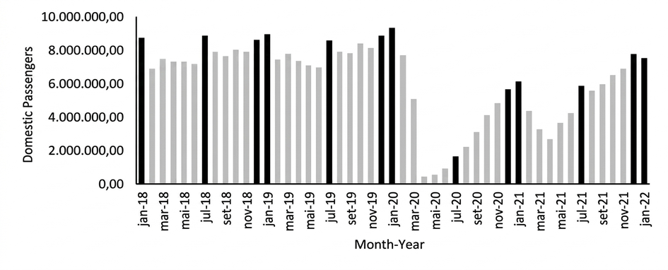
Although both models present a relatively adequate fit to explain demand behavior, it is known that the air transport market presents seasonality, with peaks in the school holiday months, which was not incorporated into these initial models. Figure 1 presents the evolution of domestic air transport demand over the last five years and shows that the months of December, January, and July have a peak compared to others, even during the pandemic, except for July 2020.
Source: ANAC (2022a).
To obtain more adjusted models that considered seasonality, new models were tested with the insertion of binary variables (or “dummies”) for each month and year in the database. This means that for each month and year, an indicator variable was created that assumes a value of 1 when the observation belongs to that period and 0 otherwise. All models proved to be significant by the F statistic and with residuals adhering to normality, according to the Shapiro-Wilk test. However, the models with all “dummies” for years and months or only for months are difficult to interpret due to the excess of variables. These models were inadequate for a broader understanding of the pandemic’s impact on demand for domestic flights, due to overfitting, that is, the estimated data adjusted excessively to the base, making the model not very robust for estimating any distinct future values.
The model with “dummies” only for the years presented more interesting coefficients, with employment level and GDP variables behaving similarly to the “absolute model without dummies” and an R² of 0.71. However, the use of a specific “dummy” for the year 2021, for example, harms the model’s generalization. After tests with variables in absolute and percentage values, the inclusion of “dummies” for months and/or years did not result in models capable of satisfactorily capturing the demand variation caused by the pandemic for future analyses.
In another effort to capture seasonal variation in demand, two other models (with absolute and percentage values) were tested with a dummy variable indicating high season in the months of December, January, and July.
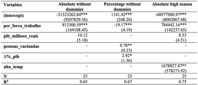
Both models proved significant by the F statistic and with residuals adhering to normality after applying the Shapiro-Wilk test, in addition to solving the overfitting problem. Furthermore, all correlations were as expected: the increase in GDP or employment level resulted in an increase in demand. The model with absolute values, referred to as “absolute high season”, did not incorporate variables related to the pandemic. The model with percentage variations showed the same results and coefficients as the “percentage without dummies” model, and the variable referring to high season was not statistically significant. After analyzing the discussed models, Table 2 compares the models that best represent demand behavior based on R2.
Table 2. Comparison of candidate models
Note. ***p < 0.001; **p < 0.01; *p < 0.05; the number format is as per the system output, therefore, decimal places are separated by a point instead of a comma.
The “absolute high season” model was chosen for presenting the highest R² (0.75), which demonstrates a better capacity to explain the behavior of demand for domestic air transport. Furthermore, the model does not include pandemic-specific variables, which increases its generalization and allows for future application. Equation 6 represents the selected model:

Where:
pass: number of domestic passengers;
employment level;
GDP: Brazil’s GDP in millions of reais;
high: binary variable indicating high season.
The interpretation of this model can be carried out as follows: with the other variables constant, a one percentage point (p.p.) increase in employment level implies an increase of 784,442 passengers transported; for each million reais more in GDP, an increase of nine passengers transported is expected; during the high season period (January, July, and December), an increase of 1,678,927 passengers transported is observed.
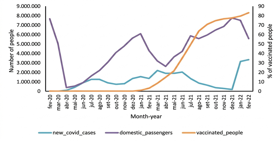
Although the variables related to the pandemic are not contemplated by the model, they show a correlation with demand (Figure 2). When there is a reduction in covid-19 cases, an increase in demand is observed. Similarly, as vaccination in the country advances, an increase in demand is verified.
Sources: ANAC (2022a), Ministry of Health (2022), and Our World in Data (2022).
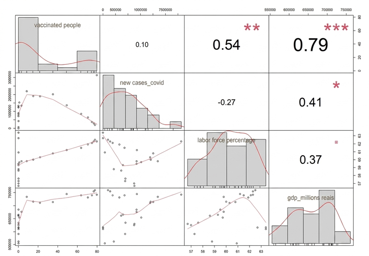
Figure 3 shows that the evolution of vaccination is highly correlated with GDP and employment levels. Furthermore, the number of new covid-19 cases is also significantly related to GDP. These links help explain the absence of specific pandemic variables in the model, as their impact is indirectly reflected by the two macroeconomic variables. In fact, this result favors the generalization of the model and its application in possible future events that similarly impact the dynamics of society and the economy.
Source: Original research results.
Gudmundsson et al.[11] highlight the historical relationship between GDP and demand for air transport. The model developed in this work confirms this relationship even during the pandemic period.
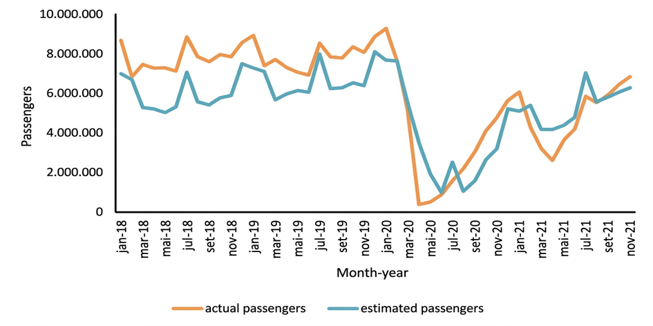
Figure 4 presents a comparison between the actual values of the quantity of domestic passengers and the values predicted by the extrapolated model for the period of the last five years. The estimated values reflected the seasonality of demand, even for data prior to the pandemic. However, the difference between the actual values and the estimated values was greater in the previous period.
Source: ANAC (2022a) and original research results.
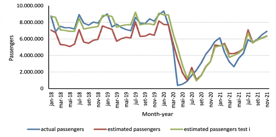
Next, a new regression was performed with data from the last five years (since January 2018), in which the variable “passengers” was defined as dependent and “GDP”, “employment level”, and “high season” as explanatory. This new model, named “test i”, showed only employment level and high season as statistically significant variables. Furthermore, its residuals did not adhere to normality. However, the results allowed for some relevant observations. Figure 5 presents a comparison between the actual number of passengers and the estimated demands.
Source: ANAC (2022a) and original research results.
The predicted demand for the pre-pandemic period by the “test i” model is closer to the actual demand compared to the original model’s estimate, and for the post-pandemic period, the difference was also not significant.
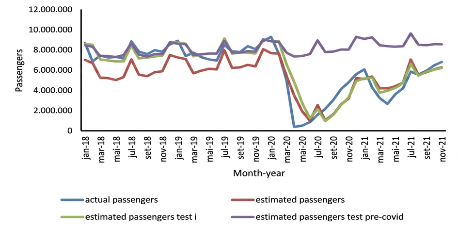
When simulating another model called “pre-covid test”, with the same variables (passengers, GDP, employment level, and high season) for the period between 2018 and 2019, the only statistically significant variables were “GDP” and “high season”. Figure 6 presents the real demand compared to the estimated demands.
Sources: ANAC (2022a) and original survey results.
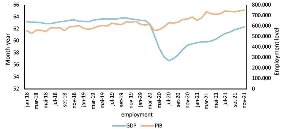
Without the inclusion of the employment level, the “pre-covid test” model does not capture the significant drop in demand after the pandemic. Figure 7 shows why the employment level is relevant when considering data after March 2020. The employment level shows a sharper drop and a more gradual recovery, a pattern similar to that observed in the demand for domestic air transport. GDP, on the other hand, shows signs of recovery two months after the declaration of the pandemic, and its drop is not as sharp. Therefore, the estimated model considers GDP as a significant variable for demand forecasting, but highlights the importance of the “employment level” in capturing the effect of crises, such as the covid-19 pandemic.
Source: Ipeadata (2022a; 2022b).
It is important to highlight some limitations of the results. In the domestic market, the absence of flight restrictions between cities allowed for a simpler demand analysis. In international contexts, regulatory factors, such as vaccine or quarantine requirements, would make the analysis more complex. Therefore, when extrapolating the results, the specific context in which the model was developed should be considered. It is also necessary to monitor possible structural changes in the labor market, such as the advancement of remote work, which may affect the model’s premises. Furthermore, the model only covers the post-pandemic recovery period and is limited to linear relationships between variables — nonlinear approaches could be explored in future studies.
In conclusion, the model offers value to airlines, airport operators, and public policymakers by guiding strategic decisions related to capacity, routes, fleet, pricing, and infrastructure investments. In addition to its utility in regular operational scenarios, it also stands out as an effective tool for dealing with disruptive events, such as pandemics or economic crises. When integrated with periodically updated economic projections or applied in simulations and stress tests, the model allows for rapid estimation of demand drops, projection of network readjustment, sizing of teams, renegotiation of contracts, and calibration of subsidy policies, which contributes to reducing the negative impacts on the sector.
The results of this study were successful in estimating demand in a way that is compatible with the effects observed during the pandemic, and the tool demonstrates potential to support continuous market monitoring and projections in similar future scenarios.
REFERENCES
[1] International Civil Aviation Organization (ICAO). 2006. Manual on air traffic forecasting. 3ed. International Civil Aviation Organization.
[2] Agência Nacional de Aviação Civil (ANAC). 2021. Em agosto, indicadores do transporte aéreo permanecem abaixo dos níveis de 2019. Disponível em: <https://www.gov.br/anac/pt-br/noticias/2021/em-agosto-indicadores-do-transporte-aereo-permanecem-abaixo-dos-niveis-de-2019>. Acesso em: 31 out. 2021.
[3] Agência Nacional de Aviação Civil (ANAC). 2022a. Dados Estatísticos do Transporte Aéreo do Brasil. Disponível em: <https://www.gov.br/anac/pt-br/assuntos/dados-e-estatisticas/dados-estatisticos/dados-estatisticos>. Acesso em: 07 abr. 2022.
[4] Ministério da Saúde. 2022. Painel Coronavírus. Disponível em: https://covid.saude.gov.br/. Acesso em: 07 abr. 2022.
[5] Our World in Data. 2022. Coronavirus Pandemic (covid-19) Vaccinations. Disponível em: https://ourworldindata.org/covid-vaccinations. Acesso em 07 abr. 2022.
[6] Agência Nacional de Aviação Civil (ANAC). 2022b. Tarifas Transporte Aéreo Passageiros Domésticos. Disponível em: https://www.gov.br/anac/pt-br/assuntos/dados-e-estatisticas/microdados-de-tarifas-aereas-comercializadas. Acesso em: 07 abr. 2022.
[7] Petrobras. 2022. Preços de Vendas de Combustíveis. Disponível em: https://petrobras.com.br/pt/nossas-atividades/precos-de-venda-de-combustiveis/. Acesso em: 17 abr. 2022.
[8] Instituto de Pesquisa Econômica Aplicada (IPEA). 2022a. Ipeadata – Taxa de participação na força de trabalho das pessoas de 14 anos ou mais de idade, na semana de referência. Disponível em: http://www.ipeadata.gov.br/Default.aspx. Acesso em: 07 abr. 2022.
[9] Instituto de Pesquisa Econômica Aplicada (IPEA). 2022b. Ipeadata – Produto Interno Bruto PIB. Disponível em: http://www.ipeadata.gov.br/Default.aspx. Acesso em: 07 abr. 2022.
[10] Oxford University Press. 2008. A Dictionary of Statistics (2 ed.). Oxford: Oxford University Press. ISBN 9780199541454. Disponível em: https://www.oxfordreference.com/display/10.1093/acref/9780199541454.001.0001. Acesso em: 04 set. 2025.
[11] Gudmundsson, S.V.; Cattaneo, M.; Redondi, R. 2020. Forecasting temporal world recovery in air transport markets in the presence of large economic shocks: The case of COVID-19. Journal of Air Transport Management 91. Disponível em: https://doi.org/10.1016/j.jairtraman.2020.102007. Acesso em: 07 abr. 2022.
COMO CITAR
Caldeira, L.K.O.; Silva, J.E. 2025. A pandemia de covid-19 e a demanda pelo transporte aéreo de passageiros em voos domésticos. Revista E&S. 6: e2023111.
ABOUT THE AUTHORS
Laís Kimie Oshiro Caldeira – Master in Transport and Public Policy and Specialist in Data Science and Analytics. Chicago, Illinois, USA.
 José Erasmo Silva – Advisor professor. Federal University of Bahia. Postgraduate Program in Accounting (PPGCONT), Avenida Reitor Miguel Calmon, s/n Canela,40231-300, Salvador, Bahia, Brazil.