
September 15, 2026
Credit Card Fraud Detection Using Neural Networks in Imbalanced Data Environments
Jefferson de Oliveira Ferreira; Lauro Marques Vicari
DOI: 10.22167/2675-6528-202602232
Article derived from a Final Course Work (TCC), with content based on the student’s original work and adapted to the editorial format of the Revista E&S with the support of the ResumeAI tool, an artificial intelligence solution developed by the Pecege Institute for textual synthesis and organization.
Summary
The growing digitalization of the financial system has made credit card transaction fraud a critical obstacle to institutional stability and customer trust. This study compared a Multilayer Perceptron (MLP) Neural Network architecture with a Logistic Regression model, used as a baseline, for fraud detection in a scenario of extreme data imbalance. A dataset of real credit card transactions was used, applying synthetic oversampling techniques (SMOTE) and the Focal Loss function to mitigate the bias of the majority class. The MLP was implemented with four dense layers, and Logistic Regression served as a reference. The experiments revealed that the Neural Network outperformed the logistic model in business metrics, achieving a Recall of 0.8553 and an F1-Score of 0.8483. Notably, the MLP reduced undue blocks (False Positives) by 23.08% compared to Logistic Regression, presenting itself as a more balanced solution between operational efficiency and user experience. However, both models faced difficulties in identifying high-value frauds due to the behavioral mimicry of the offenders. It was concluded that Neural Networks constitute a superior strategic choice for institutions seeking scalability and lower operational friction, although they require complementary business rules for high-value frauds.
Keywords: Credit Card; data science; Fraud Detection; Neural Networks; Logistic Regression.
1. Introduction
The payment ecosystem in Brazil has undergone a significant structural transformation in the last decade, driven by the widespread digitalization of financial services and the consolidation of e-commerce. In this scenario, credit cards have consolidated as the main transaction vector, registering unprecedented financial volumes, as pointed out by ABECS (2024). The migration to “Card Not Present” (CNP) modalities has brought a considerable challenge for operators, who face the refinement of digital fraud, operating in regimes of scale and speed that surpass conventional defense mechanisms.
In the national context, digital fraud has evolved into the “Fraud-as-a-Service” paradigm. Data from the Serasa Experian Indicator (2025) reveal that approximately 25% of fraud attempts detected in Brazil are related to banks and issuers, with an occurrence every 4.2 seconds. The ClearSale Fraud Map (2025) indicates that the average “ticket” for fraudulent transactions (R$ 1,083.00) is significantly higher than for legitimate transactions (R$ 549.00). This scenario compromises the viability of retail due to “chargeback”, a process in which the retailer absorbs the full loss, in addition to generating sanctions from acquirers.
Historically, fraud detection relied on traditional barriers, such as static rules and extensive manual reviews conducted by human analysts. However, these approaches lost effectiveness as the volume of transactional data grew exponentially and the sophistication of criminals increased. Fraudsters began to mimic the consumption behavior of legitimate customers to bypass previously fixed parameters, making the operational cost of maintaining large manual review teams unsustainable.
To overcome this inflexible logic, organizations have begun to implement artificial intelligence architectures capable of processing multiple variables dynamically. However, the transition to predictive models encounters challenges inherent in the nature of financial data, such as concept drift, a statistical phenomenon in which attack properties and patterns change rapidly over time (Dal Pozzolo, 2015). The dynamic nature of transactions requires algorithms that learn continuously and robust techniques to deal with extreme historical imbalance, where fraud is always a rare event in a vast ocean of legitimate data.
Related research demonstrates the analytical superiority of nonlinear models in overcoming the challenges inherent in financial data. Gouvêa et al. (2013) showed that neural architectures have superior aptitude for deciphering complex correlations and optimizing loss mitigation. Jordan and Mitchell (2015) highlight machine learning as a fundamental advancement for cybersecurity, enabling proactive threat prediction. Aggarwal (2018) and Schmidhuber (2015) explain that “Deep Learning” excels at hierarchically extracting latent, nonlinear patterns using multiple layers of abstraction. This flexibility is crucial for the precise calibration of loss functions and decision thresholds, allowing the institution to prioritize strategic security metrics, such as sensitivity (“Recall”), mitigating the drop in precision that penalizes traditional models. A misclassification resulting in a false positive, such as the undue blocking of a card, causes immediate operational friction, direct revenue loss, increased customer churn rate, and damage to the institution’s reputation, exceeding the nominal value of the chargeback the algorithm attempted to avoid.
Thus, the general objective of the present article is to develop and implement a predictive fraud detection model anchored in an “Artificial Neural Networks” architecture of the “Multilayer Perceptron” (MLP) type, and to compare it directly with a traditional Logistic Regression model (used as a “baseline”). The research seeks to validate the technical and operational effectiveness of both approaches on a representative experimental “dataset”, evaluating which algorithm delivers the best solution for addressing imbalanced data and for the strategic balance between security and consumer experience.
2. Material and Methods
For this project, a practical and data-driven (quantitative) approach was chosen. The objective was to structure a fraud detection process using deep neural networks and specific techniques to handle the scarcity of fraud observations. The code was developed in Python, employing Pandas for data manipulation and TensorFlow and Keras for modeling.
Data Source and Development Environment
The study used a “dataset” of real credit card financial transactions, obtained from the “Kaggle” repository, made available by the Machine Learning Group of Université Libre de Bruxelles and based on the studies by Dal Pozzolo (2015). The database comprises 284,807 transactions from European customers over two days. The dataset presented an extreme imbalance, with only 492 transactions classified as fraud, representing 0.172% of the total volume.
The original variables were not disclosed due to banking confidentiality regulations. In their place, 28 principal components (“features” V1 to V28) generated by a PCA (“Principal Component Analysis”) transformation were provided, with only the numerical variables Time (“Time”) and Amount (“Amount”) remaining in raw format. The presence of 28 components to represent the original variables indicates that the PCA technique was primarily employed as a cryptographic mechanism, which imposes a methodological fragility due to the absence of metadata about the original predictors, limiting the model’s explainability.
Exploratory Data Analysis and Pre-processing
An Exploratory Data Analysis (EDA) was performed using the Pandas library, confirming the integrity of the dataset and the absence of missing values. The severe data imbalance (0.172% of fraud) required a modeling strategy that went beyond the conventional, as biased algorithms would tend to ignore the minority class. For a robust analysis in extreme imbalance scenarios, metrics such as precision and recall were considered essential.
To mitigate data bias, the SMOTE (“Synthetic Minority Over-sampling Technique”) “oversampling” resampling technique was employed. SMOTE acts synthetically, identifying close neighbors of the minority class and creating new examples to balance class distribution. This technique was applied exclusively to the training set, after the separation of test data, to avoid “data leakage”. Before SMOTE, the training set contained 199,020 legitimate samples and 344 fraudulent ones. After rebalancing, the training set was equalized to 50% of each class, totaling 398,040 observations.
Table 1. Distribution of classes in the pre and post-SMOTE training set.
| Processing step | Legitimate transactions (class 0) | Fraudulent transactions (class 1) | Total of samples |
|---|---|---|---|
| Original (pre-SMOTE) | 199.020 | 344 | 199.364 |
| Balanced (post_SMOTE) | 199.020 | 199.020 | 398.040 |
Source: Original survey data
The disparity between the variables “Time” and “Amount” and the presence of “outliers” were treated with “StandardScaler”, which resizes the data to a common scale, centering the mean at zero and adjusting the standard deviation to the unit, according to Equation (1):
Z = (χ – μ) / σ (1)
where x represents the original value, μ the sample mean, and σ the standard deviation. This standardization ensures that the algorithm processes all “features” with the same hierarchical importance.
The database was subdivided into three sets: Training (70%), Validation (15%), and Test (15%). The training set was used for the convergence of synaptic weights, the validation set for monitoring performance and adjusting hyperparameters, and the test set, kept isolated, for the definitive evaluation of the model’s performance in a real-world scenario. A stratified split was used to preserve the original proportion of 0.172% of fraud in all subsamples (Training, Validation, and Test), ensuring the model’s reliability under real conditions.
Architecture and Functioning of the Neural Model
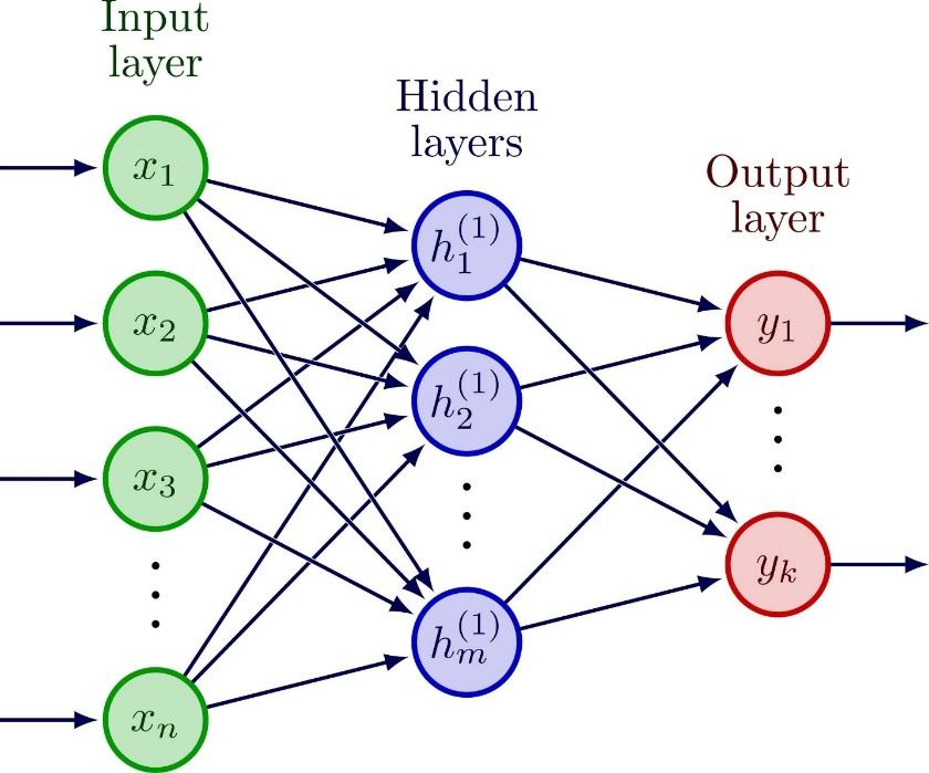
A “Multilayer Perceptron” (MLP) type Neural Network was implemented with four dense layers: an input layer with 30 neurons, three hidden layers (with 128, 64, and 32 neurons, respectively), and an output layer, according to figure 1.
Figure 1. Schematic representation of the proposed MLP Neural Network architecture
Source: Original survey data
Each neuron functions as a node that receives input signals, applies weights, and generates an activation. Dense layers are fully connected, allowing the model to learn global combinations and complex patterns. The internal functioning of each neuron is based on a linear transformation followed by a non-linear activation. The weighted sum of inputs (x) and weights (w), plus the bias (b), is calculated by:
z = (x .w) + b (2)
In the hidden layers, the ReLU (“Rectified Linear Unit”) function was applied to learn complex and non-linear patterns, accelerating the model’s convergence:
f(z) = max(0, z) (3)
To prevent “overfitting”, the hidden layers used L2 Regularization (λ = 0.0001), which adds a penalty to the loss function proportional to the square of the weights. In the output layer, the Sigmoid function was used, which compresses the result into a probability between 0 and 1:
σ(z) = 1 / (1 + e^(-z)) (4)
The learning process is based on the use of the error generated at the output as a guide for recalibrating the internal weights, through the “backpropagation” algorithm. This iterative cycle, known as the “training loop”, seeks to progressively minimize the cost function, confronting the model’s predictions with the actual targets (“labels”) to adjust the network based on gradient descent.
Figure 2. Neural network learning process
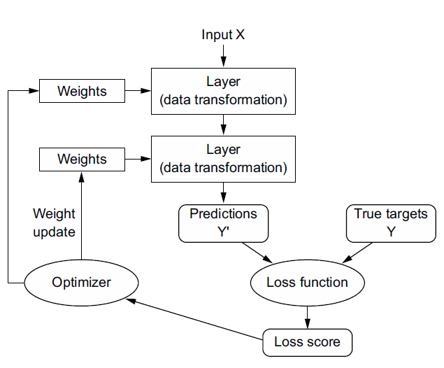
Source: Chollet (2011)
Hyperparameter tuning and experimentation
The final configuration of the neural network (128, 64, and 32 neurons) resulted from an iterative experimentation process. Table 2 presents the sensitivity metrics (“Recall”) of different architectures under the same training conditions and a “Business Approach” threshold (maximum of 50 False Positives).
Table 2. Sensitivity metrics (“Recall”) for different architectures.
| Initial architecture | Statistical Recall | Recall Business | Diagnosis |
|---|---|---|---|
| 256 neurons | 86,49% | 81,08% | Overfitting / Noise Memorization |
| 16 neurons | 86,49% | 81,08% | Underfitting / Low separation capacity |
| 128 neurons | 86,49% | 85,14% | Optimal point of generalization |
Source: Original survey data
The selected intermediate architecture (128, 64, 32 neurons) proved to be the most robust, raising business Recall to 85.14% and maximizing the identification of fraudulent transactions without compromising learning stability. The Adam (“Adaptive Moment Estimation”) algorithm was chosen as the optimizer due to its high efficiency in scenarios with sparse data and complex loss spaces, calculating adaptive learning rates for each weight individually and ensuring faster and more stable convergence. The “Early Stopping” technique was incorporated to monitor the loss on the validation set (val_loss) and interrupt training when performance gain stagnated, combating “overfitting”.
Optimization
The “Focal Loss” technique was implemented as the cost function, replacing the standard binary cross-entropy. This metric is designed to handle extreme class imbalance by focusing learning on “hard” examples (rare frauds) and penalizing the influence of legitimate transactions. The function is defined by:
FL(pt) = −αt(1 − pt)γlog(pt) (5)
where (pt) is the estimated probability for the true class, αt is the balancing factor and γ (“focusing parameter”) modulates the loss of already well-classified examples. In this study, γ = 2 and α = 0.25 were adopted, defined statically based on the literature for unbalanced data. The error was minimized through backpropagation, guided by the Adam optimizer.
A methodological differentiator was the flexibility of the classification threshold. A systematic search routine (“Threshold Moving”) was applied to identify the optimal operating point of the model, aligned with business criteria and risk appetite, and not just statistical maximization. The threshold was adjusted to keep the volume of undetected fraud (False Negatives) below 14 cases in the test set, prioritizing the containment of direct loss and minimizing False Positives.
Reference models and comparative foundation
For validation, the MLP architecture was compared with Logistic Regression, adopted as a “baseline” due to its history in “credit scoring” and fraud prevention systems. Logistic Regression attempts to separate the classes through a linear combination of the variables, mapped to a probabilistic interval by the sigmoid function:
P(y = 1|x) = 1 / (1 + e^(-(β0+β1×1+…+βnxn))) (6)
where P(y = 1|x) is the probability of a fraudulent transaction, β0 is the intercept and βi are the coefficients adjusted for each variable xi. The comparison aimed to verify if the Neural Network’s complexity would result in a real gain in “Recall” and a reduction in False Positives, and if the advanced model would extract latent information ignored by linear models. For fairness, Logistic Regression was also subjected to the threshold moving routine to achieve the same security rigor stipulated for the main model, allowing for a paired comparison of operational cost.
Use of AI in work development
During the preparation of the work, Gemini (Google) and ChatGPT (OpenAI) were used to assist in the literature search, methodology alignment, review, formatting, and translation of the abstract. The content was reviewed and edited by the author, who assumes full responsibility.
3. Results and Discussion
This section presents the results obtained by the Neural Network architecture compared to the baseline model (Logistic Regression). The discussion is not limited to statistical rigor, but seeks to translate performance metrics into business impact, evaluating the balance between security and operability.
Descriptive data analysis
Initially, the distribution of transaction values was analyzed (Figure 3). To enable density visualization and mitigate the effect of extreme outliers, transactions up to $2,000 were selected, a range that comprises approximately 99.76% of the total database. It was observed that both legitimate and fraudulent transactions are concentrated in low values, however, fraud shows a slightly higher density in microtransactions, possibly indicating card testing.
Figure 3. Probabilistic Density of Values
Source: Original research results
When converting the original time to a 24-hour cycle (Figure 4), it was observed that legitimate transactions follow the standard commercial rhythm. In contrast, fraud maintains a relevant density during the early morning hours (between 2 AM and 6 AM), a period of lower active user surveillance, which characterizes the temporal factor as a strong indicator of anomaly. The proportional increase in attempts during lower transactional volume hours suggests an attempt to exploit windows with lower monitoring sensitivity. Therefore, the inclusion of this feature offers the neural network a valuable contextual dimension to differentiate typical from atypical behavior.
Figure 4. Transaction density per hour
Source: Original research results
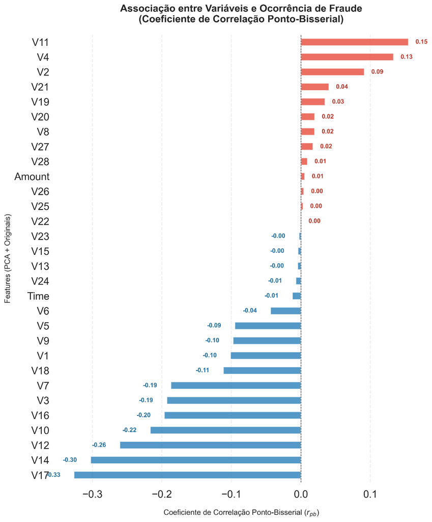
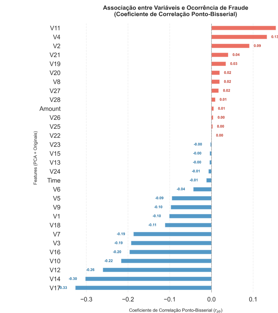
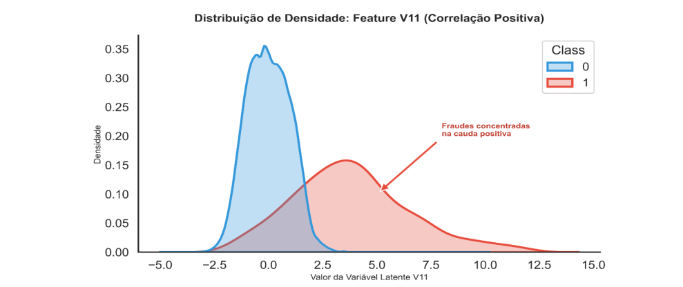
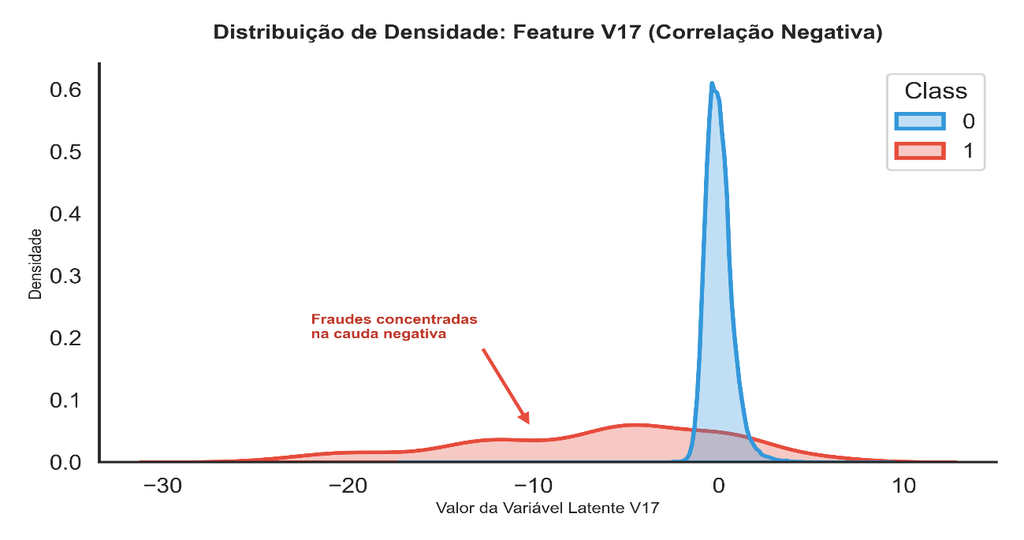
Continuing the relevance analysis, Figure 5 presents the association between latent variables (V1 to V28) and the occurrence of fraud, using the point-biserial correlation coefficient. The mapping revealed that variables such as V17 (negative) and V11 (positive) are the main indicators of fraud. Variables like V17, V14, and V12 exhibit more pronounced negative associations, indicating that lower values in these dimensions increase the probability of fraudulent transactions. On the other hand, V11 and V4 show the largest positive associations, acting as risk indicators as their values increase. The density distributions of the variables with the greatest impact were examined individually, visually confirming the separation between classes.
Figure 5. Correlation between the variables
Source: Original research results
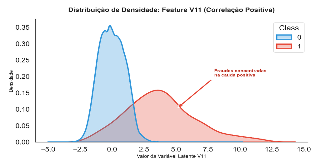
In Figure 6, the behavior of the variable V11 (positive correlation) is observed, where the displacement of the fraud data mass (in red) to the right of the normal transaction curve is clear, ratifying V11 as a robust predictor. Similarly, Figure 7 details the variable V17 (negative correlation), where the density of frauds is severely concentrated in the left tail (negative values), as predicted by the point-biserial coefficient. The differential of the MLP Neural Network lies in its ability to process these polarities in a multivariate manner, capturing complex fraud patterns that escape simple linear association metrics.
Figure 6. V11 density distribution
Source: Original research results
Figure 7. V17 density distribution
Source: Original research results
Monitoring of Metrics and Identification of “Overfitting”
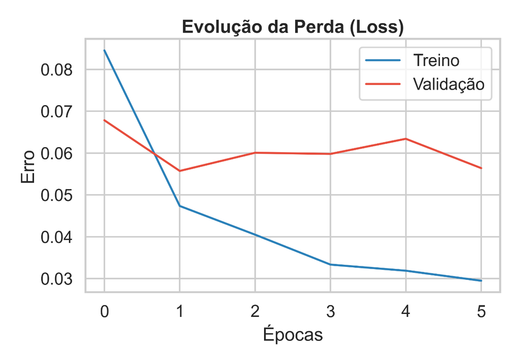
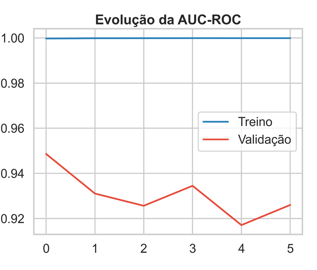
The neural network performance evaluation began with monitoring the learning curves over the training epochs, as detailed in Figures 8 and 9. The results revealed a classic scenario of early overfitting. In the Loss graph, it was observed that while the training error decreased steadily, the validation curve showed an upward and unstable inflection after the first epoch, indicating that the model began to adjust excessively to the noise in the training set. This behavior was corroborated by the evolution of the AUC-ROC metric, where the model quickly reached the maximum score (AUC-ROC = 1.00) on the training set but failed to maintain stability on the validation data, oscillating between 0.91 and 0.94. This disparity between the curves confirmed that, despite the L2 regularization techniques, the network tended to memorize historical patterns at the expense of generalization. Therefore, interrupting the training via Early Stopping proved fundamental to preserving the artifact’s practical utility, triggering the stop at the 6th epoch to ensure the model ceased learning at its point of greatest balance.
Figure 8. Evolution of loss
Source: Original research results
Figure 9. Evolution of AUC (area under curve) during training
Source: Original research results
Comparative analysis of performance metrics
To validate the effectiveness of the proposed architecture, a direct comparison was made between the MLP Neural Network and the Logistic Regression baseline. Although the logistic model presented solid performance for evident transactional patterns, the Neural Network demonstrated a refined superiority by capturing non-linear nuances that escape traditional regression. Table 3 consolidates this technical disparity.
Table 3. Comparison of metrics
| Metric | Logistic Regression | Neural Network (MLP) | Variation (%) | Variation (p.p) |
|---|---|---|---|---|
| “Recall” (sensitivity) | 0,8378 | 0,8514 | 1,60 | + 1,36 |
| Precision | 0,6596 | 0,7079 | 6,82 | + 4,83 |
| F1-Score (Balance) | 0,7381 | 0,7730 | 4,51 | + 3,49 |
| AUC-ROC (Global) | 0,9658 | 0,9584 | -0,77 | – 0,74 |
| False Negatives (FN) | 12 | 11 | -9,09 | – 1 |
| Improper Lockouts (FP) | 32 | 26 | -23,08 | – 6 |
Source: Original research results
The most relevant data for the financial operation is the Recall of 0.8514 achieved by the Neural Network. In the context of payment methods, Recall is the sovereign metric, as it reflects the system’s ability to minimize False Negatives. The 9.09% reduction in missed fraud (from 12 to 11 cases in the test) represents direct savings in chargeback costs. In parallel, the significant drop of 23.08% in undue blocks (False Positives) is a critical gain in user experience, avoiding unnecessary friction with legitimate customers.
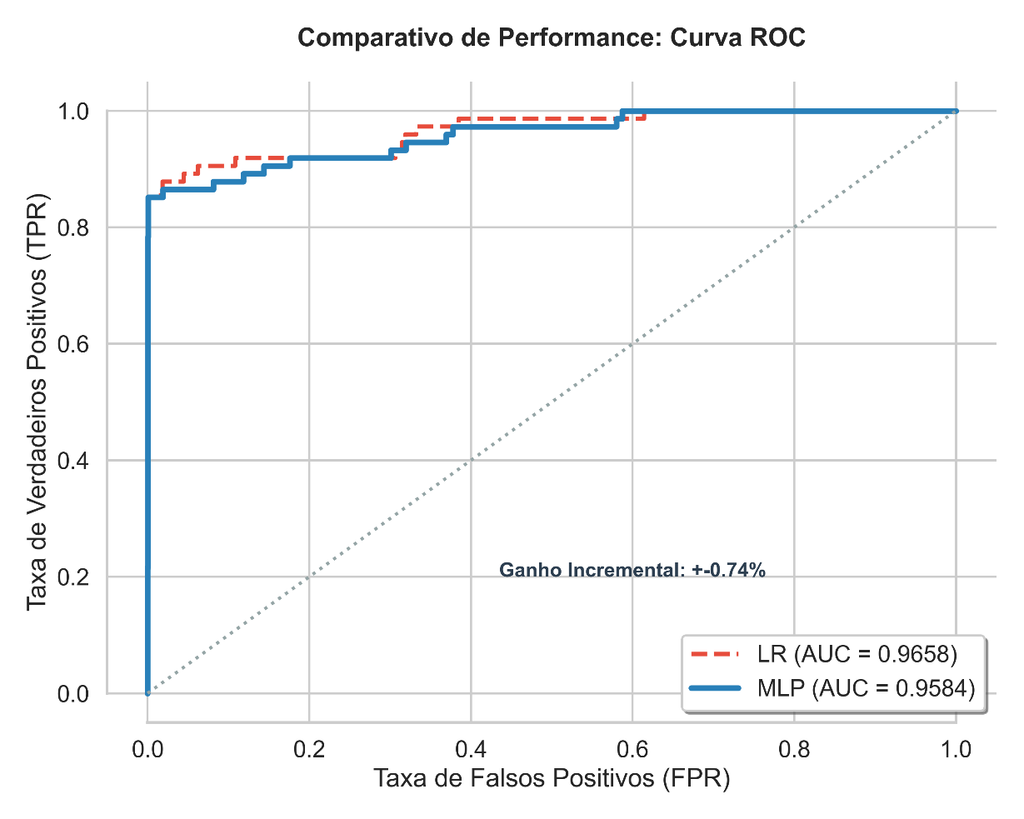
The class separation capability is visualized in the comparison of the ROC Curves (Figure 10). Both trajectories exhibit an ideal proximity to the upper-left corner of the graph, attesting to the high quality of the developed models. Although Logistic Regression boasts a slightly superior global AUC-ROC metric (0.9658), this value reflects a theoretical average performance encompassing all possible decision thresholds, including extreme cutoff points that would never be adopted in a real-world scenario. In the region of practical business interest, where the goal is to maximize fraud detection with the least possible impact on undue blocks, the Neural Network trajectory shows itself to be equivalent and, in certain intervals, more stable. This stability means that the model can sustain a high hit rate without suffering a disproportionate and abrupt increase in false alarms, confirming that the Deep Learning-based architecture is highly competitive and robust for decoding the complexity of latent variables in the credit card ecosystem.
Figure 10. ROC Curve Comparison: Logistic Regression vs. MLP Neural Network
Source: Original research results
Operational performance and threshold optimization
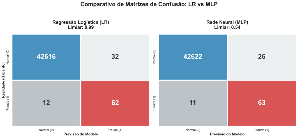
To evaluate the model by simulating the production environment, the confusion matrix was applied to the test base, ensuring the impartiality of the predictions. In scenarios of extreme imbalance, the analysis of this matrix is indispensable for quantifying the exact volume of correct predictions (True Positives) against the critical financial risk of undetected fraud (False Negatives). The high class separation capacity demonstrates the success of the adopted hybrid approach. The SMOTE algorithm intervened in the preprocessing, mitigating the deficit of the base by synthesizing new samples for the minority class. In contrast, Focal Loss acted directly on the neural network training, calibrating the cost function to prioritize borderline and difficult-to-classify fraud. This dual strategy enabled the construction of a robust decision boundary. The visual result of this strategy can be observed in Figure 11, which presents the comparison of the confusion matrices. It was noted that the MLP achieved a significant reduction in False Positives compared to the logistic baseline, maintaining an equivalent level of security in detecting real fraud.
Figure 11. Confusion matrices – Test set
Source: Original research results
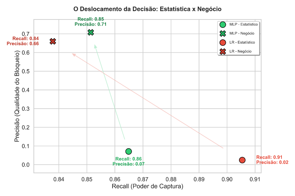
A central point of this stage was the rejection of the standard statistical threshold of 0.5. As illustrated in Figure 12, the strategic calibration of the trade-off between Precision and Sensitivity (Recall) allowed for the identification of the optimal operating point for the real-world scenario. This decision prioritized operational sustainability, establishing a strict ceiling for the volume of False Positives to avoid undue customer blocking, in exchange for rigorous maintenance of high-impact fraud capture. Figure 12 illustrates the fundamental dilemma between Precision (Blocking Quality) and Recall (Capture Power) in statistical and business approaches. In the purely statistical approach, both models aim for maximum capture (Recall), resulting in high fraud detection (LR = 0.91; MLP = 0.86), but with unacceptably low precision (LR = 0.02; MLP = 0.07), generating an unsustainable volume of false positives. By adopting a business perspective, decision thresholds are adjusted to balance fraud capture with operational cost and customer experience. The analysis of the graph reveals the operational superiority of the Neural Network model [MLP]. While the Logistic Regression model [LR] undergoes a severe trade-off to achieve an operational Precision of 0.66, significantly sacrificing Recall (dropping to 0.84), the MLP model demonstrates remarkable efficiency. The shift of the MLP to the business strategy achieves superior Precision (0.71) with almost no loss of Recall (dropping only from 0.86 to 0.85). This characteristic proves that the MLP model is more robust and capable of finding optimized operating points, maximizing fraud capture with minimal operational friction. This double gain validates the hypothesis that the Neural Network’s ability to process non-linear patterns through its hidden layers allows for a more refined separation in the decision space, overcoming the intrinsic limitations of linear models in complex banking data.
Figure 12. The Decision Displacement: Statistics x Business
Source: Original research results
Statistical analysis of errors and value disparity
To deepen the discussion on the model’s effectiveness, a comparative analysis was conducted between detected frauds and those the model failed to identify. Reversing the mathematical standardization allowed observation of the real transaction values in their original magnitudes. The analysis revealed a critical behavioral pattern, as shown in Figures 13 and 14. In both models, lost frauds (False Negatives) presented a significantly higher median value than those successfully detected. In Logistic Regression, detections primarily occurred in low-value transactions (median of $2.00), while failures were concentrated in operations with a median of $231.64. In the Neural Network, the phenomenon was analogous: the model was effective in capturing small-value frauds but encountered greater difficulty in transactions with a median of $276.17. This scenario raises a warning about the model’s applicability: frauds that generate the largest financial losses are managing to bypass the detection system due to the behavioral mimicry of criminals who imitate the consumption of high-ticket legitimate customers. There is no significant financial difference between the architectures regarding the capture of major fraudsters, as both algorithms allow these transactions to pass. The true trade-off between the methodologies lies in operational efficiency with the customer base, where the Neural Network (MLP) acts more cleanly, generating 18.7% fewer undue blocks compared to the baseline.
Figure 13. Baseline Financial Impact: MLP
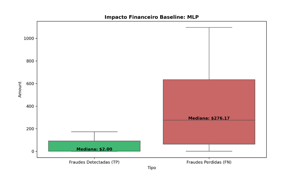
Source: Original research results
Figure 13. Baseline Financial Impact: Logistic Regression
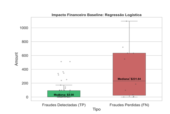
Source: Original research results
The present investigation demonstrated that the Multilayer Perceptron (MLP) Neural Network architecture offers real gains over traditional Logistic Regression in credit card fraud detection, especially in imbalanced data environments. The strategic implementation of synthetic oversampling (SMOTE) in conjunction with the Focal Loss loss function optimized the model’s resistance to the majority class bias, resulting in high levels of F1-Score and Precision, as well as training stability that minimizes oscillations in generalization capacity. The MLP showed an 18.7% reduction in False Positives compared to Logistic Regression, translating into greater operational efficiency and a better user experience. However, error analysis revealed that the highest nominal value frauds still manage to bypass the neural network barrier due to the behavioral mimicry of criminals, indicating that the ability to predict the mathematical probability of an event must be complemented by mechanisms that weigh the absolute financial risk involved.
4. Conclusion
This study aimed to develop and compare a predictive model for credit card transaction fraud detection, using a Multilayer Perceptron (MLP) Neural Network architecture against a Logistic Regression baseline, focusing on handling imbalanced data and the strategic balance between security and user experience. It was found that the MLP demonstrated superiority in business metrics, achieving a Recall of 0.8514 and a 23.08% reduction in undue blocks (False Positives) compared to Logistic Regression. The strategic application of synthetic oversampling techniques (SMOTE) and the Focal Loss loss function was fundamental to mitigating the bias of the majority class and optimizing model robustness. This approach resulted in high levels of F1-Score and Precision, as well as training stability that minimized oscillations in generalization capability. The Neural Network, therefore, constitutes a superior strategic choice for financial institutions aiming for scalability and reduced operational friction, without compromising security.
However, the error analysis revealed that both models faced difficulties in identifying high nominal value frauds, attributed to the behavioral mimicry of criminals, who manage to bypass the detection network. This limitation indicates the need to complement mathematical predictive capacity with mechanisms that weigh the absolute financial risk involved. Additionally, the use of a static dataset restricted the view on the dynamic and temporal nature of frauds, and the PCA transformation imposed a fragility in the causal explainability of the original variables. As future developments, it is suggested to implement secondary business rules focused on containing high-value anomalies and transitioning to recurrent architectures, such as LSTMs or RNNs, capable of interpreting the cardholder’s history as a logical and chronological sequence, improving detection in “Concept Drift” scenarios.
Bibliographic References
ABECS. 2025. Balanço do setor de meios eletrônicos de pagamento: resultados 2024. Associação Brasileira das Empresas de Cartões de Crédito e Serviços, São Paulo, SP, Brasil. Disponível em: Acesso em: 05 fev. 2026.
Aggarwal, C.C. 2018. Neural Networks and Deep Learning. Springer, Cham, Suíça. Disponível em: . Acesso em: 12 out. 2025.
Cholet, F. 2021. Deep learning with python. 2ed. Manning, New York, EUA.
ClearSale. 2025. Mapa da Fraude. Disponível em: Acesso em: 10 jan. 2026.
Dal Pozzolo, A. 2015. Adaptive Machine learning for credit card fraud detection. Tese, Ph.D. em Ciência da Computação, Université Libre de Bruxelles. Disponível em < http://di.ulb.ac.be/map/adalpozz/pdf/Dalpozzolo2015PhD.pdf>
Gouvêa, M.A.; Gonçalves, E.B.; Mantovani, D.M.N. 2013. Análise de risco de crédito com aplicação de regressão logística e redes neurais. Contabilidade Vista & Revista 24(4): 96-123. Disponível em: < https://www.redalyc.org/pdf/1970/197033497006.pdf > Acesso em: 12 out. 2025.
Jordan, M.I.; Mitchell, T.M. 2015. Machine learning: Trends, perspectives, and prospects. Science 349(6245): 255-260. Disponível em: Acesso em: 12 out. 2025.
Schmidhuber, J. 2015. Deep learning in neural networks: An overview. Neural Networks 61(1): 85-117. Disponível em: . Acesso em: 15 out. 2025.
Serasa Experian. 2025. Record: Almost 7 million fraud attempts were registered in the 1st quarter of 2025; the banking sector is the main target. Available at: Accessed on Jan. 10, 2026.
Article originating from the Course Conclusion Work of the Specialization in Data Science and Analytics of the MBA USP/Esalq
To learn more about the course, click here and access the MBX Academy platform