Article

Kleyton Santos Rodrigues de Sousa; Luiz Henrique Lino de Oliveira

DOI: 10.22167/2675-6528-202603755

Article derived from a Term Paper (TCC), with content based on the student’s original work and adapted to the editorial format of the E&S Magazine with the support of the ResumeAI tool, an artificial intelligence solution developed by the Pecege Institute for textual synthesis and organization.

Summary

Aggregate default in the Brazilian financial system is a crucial indicator of credit risk, whose prediction is regulated by CMN Resolutions n.° 4.557/2017 and 4.966/2021 for the prospective measurement of expected losses. Aggregate default was modeled and predicted using the SARIMAX model, projecting its trajectory until December 2026 under optimistic, base, and pessimistic scenarios. 164 monthly observations (July/2012 to February/2026) and macroeconomic variables such as unemployment, Selic, IPCA, IBC-Br, and household debt were used. The specification with contemporaneous variables was selected based on information criteria and coefficient stability, and residual diagnostics confirmed statistical adequacy, with an MAPE of 3.12%. Historical default ranged between 4.33% and 7.64%. The estimation identified unemployment (β = 0.2534; p < 0.001) and Selic (β = 0.2128; p < 0.001) as the main positive determinants, with strong temporal persistence (AR(1) = 0.8965). Selic showed increasing correlation with default (r = 0.62 at lag 12), while unemployment demonstrated a contemporaneous effect (r = 0.33). Projections indicated default between 6.30% and 7.98% in December 2026, with a range of 1.68 percentage points, highlighting direct implications for provisioning in financial institutions.

Keywords: Unemployment; Predictive modeling; Monetary policy; Loss provision; Time series.

1. Introduction

Aggregate default in the Brazilian financial system, defined as the proportion of the outstanding balance with delays exceeding ninety days in relation to the total balance of credit operations, represents one of the main credit risk indicators monitored by the Central Bank of Brazil (BCB, 2024). The forecast of this indicator is a formal regulatory requirement, established by Resolutions of the National Monetary Council (CMN) number 4.557/2017 and 4.966/2021. These regulations impose a forward-looking approach in the measurement of expected losses, demanding the consideration of reasonable projections on future economic conditions (CMN, 2017; CMN, 2021; Basel Committee on Banking Supervision, 2015).

The behavior of non-payment is intrinsically associated with macroeconomic conditions. When unemployment increases, household income decreases and the ability to honor debts deteriorates. Similarly, the rise in interest rates makes installments on indexed contracts more expensive and refinancing of debts more burdensome. The slowdown in economic activity, in turn, compromises both the income flow and the cash generation of companies (Mishkin, 2016; Bernanke; Gertler, 1989). It is important to note that these transmission mechanisms are not instantaneous, and the impact of economic shocks on non-payment typically manifests with lags of weeks to months, which highlights the importance of understanding the temporal behavior of these variables for predictive modeling (Gujarati; Porter, 2011; Enders, 2015).

For financial institutions, non-payment directly impacts the constitution of provisions for expected losses, affecting financial results and the capacity to grant new credit (BCB, 2024; Basel Committee on Banking Supervision, 2015). For credit takers, it results in negative credit reporting, restricted access to financing, and increased future credit costs. At the macroeconomic level, systemic non-payment shocks can amplify recessionary cycles by restricting aggregate credit, as documented by Boudoukh et al. (2009) and Jiménez et al. (2008) in international contexts, and by Barbosa (2007) in the Brazilian case, where household income commitment to debt reached historically high levels in the last decade. Non-payment in the Brazilian financial system varied between 4.33% and 7.64% in the period from July 2012 to February 2026, with a historical average of 5.96%, evidencing the volatility and relevance of the issue.

The literature on default prediction is vast and multidisciplinary (Thomas; Crook; Edelman, 2017; Bellotti; Crook, 2009). Previous studies, such as Barbosa (2007), applied Autoregressive Integrated Moving Average (ARIMA) models to aggregate default, demonstrating the influence of the economic cycle on credit risk. Jiménez et al. (2008) and Boudoukh, Richardson, and Whitelaw (2009) showed how macroeconomic shocks affect the probability of default at different time horizons. More recently, Machado (2025) conducted a comparative analysis between ARIMA, ARIMA with exogenous variables (ARIMAX), neural networks, and hybrid models applied to the default of Brazilian financial institutions. The choice of time series models with exogenous variables, such as SARIMAX, is justified by their ability to capture the temporal persistence of the indicator and incorporate the influence of macroeconomic factors, offering interpretability and suitability for prospective purposes.

Given the importance of default as an indicator of credit risk and the regulatory requirement for prospective approaches, the ability to accurately predict its trajectory becomes fundamental for risk management and provisioning. The objective of this work is to model and predict the aggregate default of the Brazilian financial system using the SARIMAX(1,0,1) model with contemporary exogenous macroeconomic variables, projecting its trajectory from July 2012 to December 2026 under optimistic, base, and pessimistic scenarios, in order to support risk analyses and provisioning in compliance with the current regulatory framework.

2. Material and Methods

The data were obtained exclusively from official public sources. Monthly macroeconomic series were collected via the Application Programming Interface [API] of the Central Bank of Brazil’s Time Series Management System [SGS], and the unemployment rate was extracted from the Continuous National Household Sample Survey [PNAD] of the Brazilian Institute of Geography and Statistics [IBGE]. The sample covers the period from July 2012 to February 2026, totaling 164 monthly observations after pre-processing. The dependent variable — total financial system default (BCB, series 25464) — is defined as the proportion of the balance with delays exceeding 90 days in relation to the total balance of credit operations, expressed as a percentage. Data treatment included: removal of missing observations in the default series; linear interpolation for periods without observations in unemployment, due to the quarterly periodicity of the Continuous PNAD; creation of lagged variables (1, 3, and 6-month lags) during pre-processing to ensure that all observations used had a complete history of macroeconomic variables, which resulted in the sample starting in July 2012. All data processing, SARIMAX model estimation, and diagnostic tests were conducted in Python, using the “statsmodels” library for statistical modeling and the “matplotlib” and “seaborn” libraries for generating the visualizations presented in this work.

Five exogenous variables were selected based on economic relevance and literature evidence, all included in the model in their contemporary versions. Table 1 consolidates the characteristics of all variables in the dataset used in the model.

Table 1: Description of the Dataset Variables (Jul/2012-Feb/2026).

Source: Own elaboration based on BCB/SGS and IBGE/PNAD Contínua.

Variable	Description	Unit	Source / Series	Periodicity	Role in the model
Nonpayment	Proportion of the outstanding balance with delay >90 days over the total credit balance of the SFN	%	BCB / Series 25464	Monthly	“TARGET” (dependent variable)
Unemployment	Unemployment rate of the workforce [PNAD Continuous]	%	IBGE / Continuous PNAD	Quarterly (interpolated)	Contemporary exogenous
Selic	Average monthly base interest rate (cost of credit)	% a.a.	BCB / Series 432	Monthly	Contemporary exogenous
IPCA 12 months	12-month accumulated inflation (pressure on real income)	%	BCB / Series 13522	Monthly	Contemporary exogenous
IBC-Br	BCB’s Economic Activity Index (“monthly proxy” for GDP)	Index	BCB / Series 24363	Monthly	Contemporary exogenous
Household Debt	Household debt commitment in relation to income (financial vulnerability)	%	BCB / Series 20682	Monthly	Contemporary exogenous

As a complementary exploratory analysis, cross-correlations [CCF – “Cross-Correlation Function”] were calculated between nonpayment and each macroeconomic variable for lags of 0 to 12 months. The objective of this analysis is to characterize the transmission time horizon between macroeconomic indicators and credit risk, contributing to the interpretation of the model’s results. It is important to note that this analysis is exploratory: the exogenous variables were included in the SARIMAX model in their contemporary forms, as specified by the modeling code.

The choice of the SARIMAX(1,0,1) model was based on three criteria. From a theoretical standpoint, the model combines the autoregressive [AR] structure that captures the strong temporal persistence of default with contemporary macroeconomic exogenous variables, making it suitable for the prospective purpose of the work: to generate forecasts under alternative scenarios of economic conditions. From a statistical standpoint, the ARIMA(1,0,1) specification was selected based on the lowest AIC (6.03) and BIC (30.73) information criterion values among the tested combinations. From a comparative standpoint, SARIMAX has the additional advantage of interpretability: each coefficient has direct economic meaning, an attribute valued in regulatory contexts. The model formulation is:

yt = c + β1 · unemploymentt + β2· selict + β3· ipcit +ẞ4· ibcbrt +ẞ5· endividt + p1 • (yt – 1 — μt − 1) + 01· εt − 1 + ɛt

where the parameters were estimated by the maximum likelihood method with [OPG] covariance.

After the estimation, three scenarios were defined for projection until December 2026, anchored in the economic outlooks available in the period of elaboration of this work (March 2026). The base scenario was calibrated from the medians of the Boletim Focus of the Central Bank of Brazil (BCB, 2026a), which projected Selic at 12.50% by the end of 2026, IPCA at 4.17%, and average annual unemployment of approximately 5.8% for the period — values used as a central reference and adjusted to the levels of the variable along the model’s projection horizon. The optimistic and pessimistic scenarios were constructed as symmetric deviations from the base scenario, representing trajectories of monetary easing and labor market convergence to historically favorable levels (optimistic scenario), and fiscal deterioration, inflationary persistence, and interest rate hikes above projections (pessimistic scenario), in line with the methodology for constructing stress scenarios adopted in credit risk analyses (BCB, 2024). The optimistic scenario assumes a drop in unemployment to 4.5%, Selic at 8.5%, IPCA at 3.5%, IBC-Br at 145, and indebtedness at 120. The base scenario considers unemployment at 6.0%, Selic at 12.5%, IPCA at 5.0%, IBC-Br at 140, and indebtedness at 125. The pessimistic scenario contemplates unemployment at 9.0%, Selic at 16.0%, IPCA at 7.0%, IBC-Br at 120, and indebtedness at 150. In all scenarios, variables were kept constant throughout the projection horizon, which constitutes a methodological simplification to be considered in the interpretation.

3. Results and Discussion

Exploratory data analysis

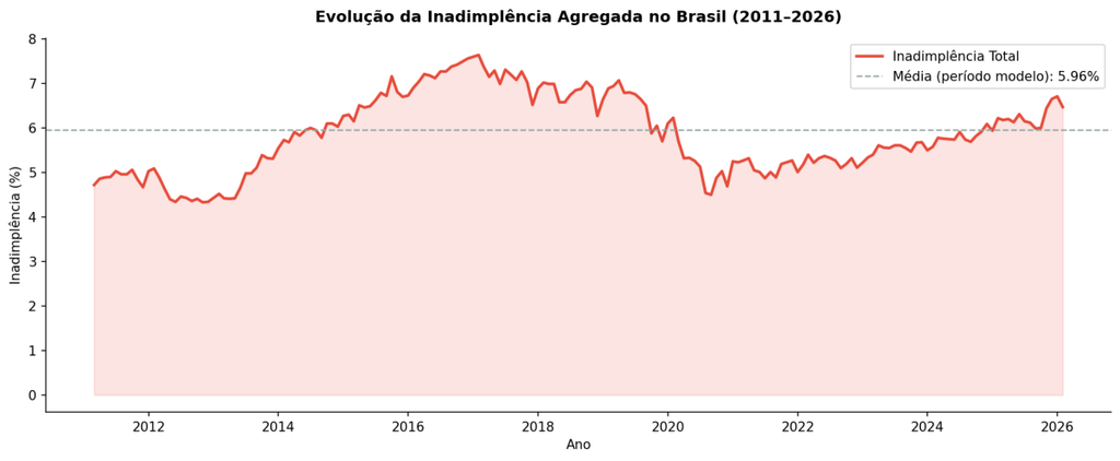
The historical evolution of aggregate non-payment in the Brazilian financial system, as shown in Figure 1, exhibited cyclical behavior with three distinct phases. Between 2012 and 2017, an upward cycle was observed, attributed to the worsening macroeconomic conditions during the 2015–2016 recession, with increased unemployment, a drop in real income, and deterioration of consumer confidence. The peak in 2020 was associated with the COVID-19 pandemic, which caused a sharp contraction in economic activity, although emergency policies temporarily acted to curb non-payment. From 2021 onwards, a new upward trend in non-payment was observed, mainly due to the monetary tightening cycle, which increased the cost of credit and raised households’ income commitment.

In the analyzed period (July 2012 to February 2026), nonpayment varied between 4.33% and 7.64%, with an average of 5.96% and a standard deviation of 0.87 percentage points. The persistence of nonpayment above the historical average in the post-2020 period suggests a possible structural change in credit conditions, related to higher household leverage and a prolonged environment of high interest rates. The range of 3.3 percentage points between the minimum and maximum values reinforces the relevance of models that incorporate macroeconomic variables for credit risk forecasting.

Figure 1: Evolution of Aggregate Nonpayment in Brazil (2011–2026). Dashed line indicates the model period average (5.96%).

Source: Own elaboration based on BCB/SGS (2026).

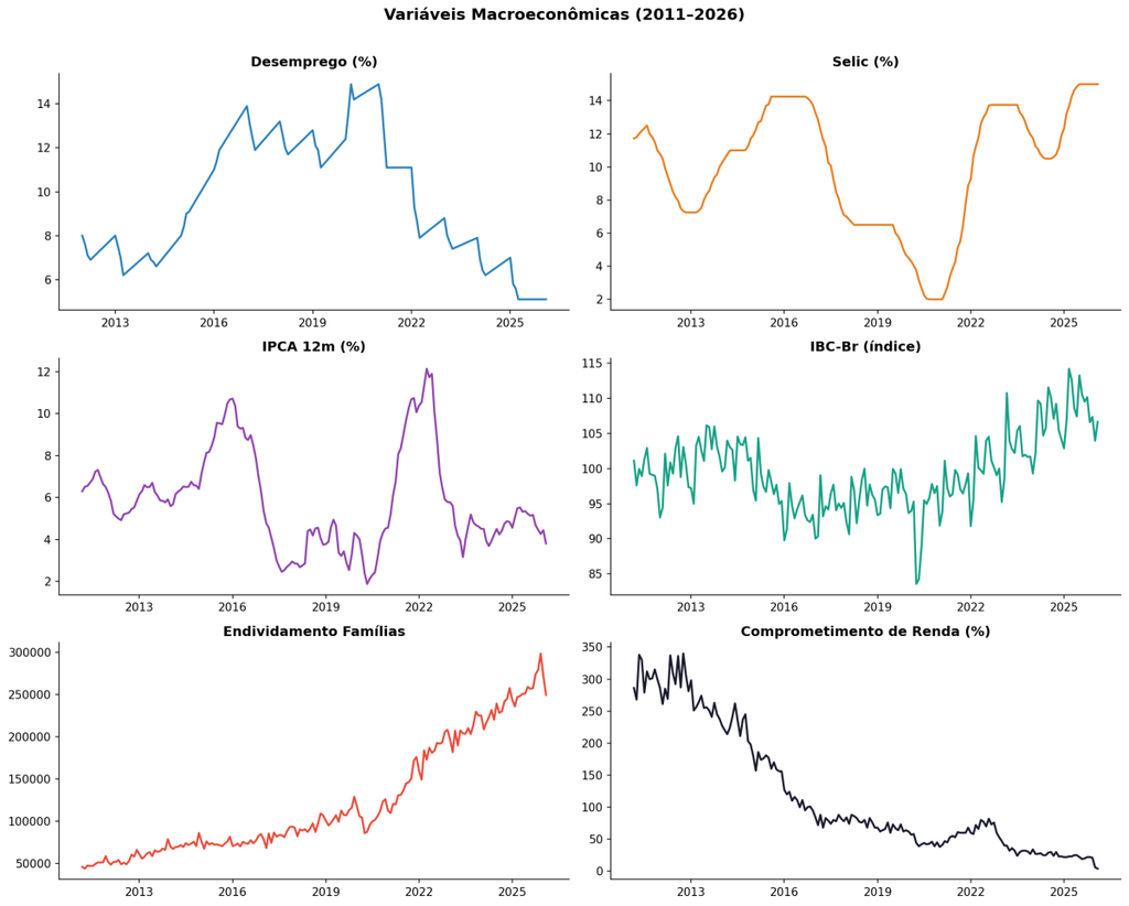
Figure 2 illustrates the evolution of the macroeconomic variables used in the model. Unemployment varied from 5.1% to 14.9%, peaking in 2017. The Selic rate fluctuated between 2.0% and 15.0%, reaching a historic low in 2020 and showing a sharp increase between 2021 and 2023. The 12-month IPCA varied between 1.88% and 12.13%, peaking in 2022. The IBC-Br varied between 83.57 and 114.20, with a drop in 2020 and subsequent recovery. The joint visualization of these series reveals that the pandemic period concentrated the greatest shock in the IBC-Br and the historic low of the Selic, preceding the inflationary escalation of 2021–2022. Between 2023 and 2025, the Selic remained at high levels even with the deceleration of the IPCA, indicating a scenario of high real interest rates that pressures the cost of household debt. This interaction between variables justifies their joint inclusion in the SARIMAX model.

Figure 2: Evolution of Macroeconomic Variables Used in the Model (2011–2026).

Source: Own elaboration based on BCB/SGS and IBGE/PNAD Contínua (2026).

Table 2 presents the descriptive statistics of the variables. Default had a mean of 5.96% and a standard deviation of 0.87. The average unemployment was 9.66%, with a standard deviation of 2.88. Selic presented a mean of 9.85% and a standard deviation of 3.85. The 12m IPCA had a mean of 5.81% and a standard deviation of 2.43. The IBC-Br registered a mean of 99.51 and a standard deviation of 5.61. Household indebtedness had a mean of 129,019 and a standard deviation of 67,247.

Table 2. Descriptive Statistics of Variables (Jul/2012–Feb/2026, N=164)

Variable	Description	Unit	Source / Series	Periodicity	Role in the model
Nonpayment	Proportion of the outstanding balance with delay >90 days over the total credit balance of the SFN	%	BCB / Series 25464	Monthly	“TARGET” (dependent variable)
Unemployment	Unemployment rate of the workforce [PNAD Continuous]	%	IBGE / Continuous PNAD	Quarterly (interpolated)	Contemporary exogenous
Selic	Average monthly base interest rate (cost of credit)	% a.a.	BCB / Series 432	Monthly	Contemporary exogenous
IPCA 12 months	12-month accumulated inflation (pressure on real income)	%	BCB / Series 13522	Monthly	Contemporary exogenous
IBC-Br	BCB’s Economic Activity Index (“monthly proxy” for GDP)	Index	BCB / Series 24363	Monthly	Contemporary exogenous
Household Debt	Household debt commitment in relation to income (financial vulnerability)	%	BCB / Series 20682	Monthly	Contemporary exogenous

Source: Own elaboration (Python/pandas, 2026).

The cross-correlation function (CCF) analysis for lags of 0 to 12 months revealed distinct behaviors. Unemployment showed a more expressive positive correlation at lag 0 (r = 0.33), with a predominantly contemporaneous effect. Selic showed an opposite pattern, with increasing correlation with the lag, reaching r = 0.62 at lag 12, reflecting the gradual transmission mechanism of credit cost. The IBC-Br showed a more expressive negative correlation at lag 0 (r = -0.27), while the IPCA had a correlation close to zero in the short term (r = -0.09 at lag 0), growing modestly at longer lags. This analysis reinforces that Selic and unemployment are the most relevant macroeconomic vectors for the dynamics of Nonpayment, acting with distinct time horizons.

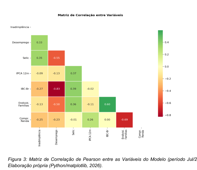
Pearson’s correlation matrix (Figure 3) confirmed a positive correlation between nonpayment and unemployment (r = 0.33) and with Selic (r = 0.35), as well as a negative correlation with IBC-Br (r = -0.27). The strong negative correlation between Selic and unemployment (r = -0.55) reflected the Brazilian monetary policy cycle, while the correlation between IBC-Br and unemployment (r = -0.83) highlighted the classic relationship between economic activity and the labor market. The correlation between household debt and Selic (r = -0.50) suggested that debt tended to accumulate during periods of low interest rates. These interrelationships signal the presence of moderate multicollinearity among the regressors, which justifies caution in the isolated interpretation of each coefficient.

Figure 3: Pearson Correlation Matrix between Model Variables (period Jul/2012–Feb/2026).

Source: Own elaboration (Python/matplotlib, 2026).

The descriptive analysis of the distributions indicated that nonpayment exhibited a median around 6%, with a compact interquartile range (approximately 5.3% to 6.5%) and absence of extreme outliers, suggesting that the series remained within a relatively stable interval. Unemployment showed a median close to 9%, with upper outliers above 14%, corresponding to the peak of the 2017 recession. Selic exhibited the largest interquartile range (from approximately 6.5% to 13.5%), with lower outliers close to 2%, corresponding to the period of historically low rates during the pandemic. The 12m CPI showed a median close to 5% and three upper outliers above 10%, capturing the inflationary episodes of 2015–2016 and 2021-2022.

Model Estimation and Coefficient Analysis

The SARIMAX(1,0,1) model was estimated over 164 monthly observations. The choice of the model was based on theoretical, statistical, and comparative criteria. Theoretically, the model combines the autoregressive structure, which captures the strong temporal persistence of default, with contemporary macroeconomic exogenous variables, being suitable for generating forecasts under alternative scenarios. Statistically, the ARIMA(1,0,1) specification was selected based on the lowest AIC (6.03) and BIC (30.73) information criterion values among the tested combinations. Comparatively, SARIMAX offers the advantage of interpretability, with each coefficient having direct economic meaning. The model formulation is: yt = c + β1 · unemployt + β2· selt + β3· ipct + ẞ4· ibcrt +ẞ5· endivt + φ1 • (yt – 1 — μt − 1) + θ1· εt − 1 + ɛt.

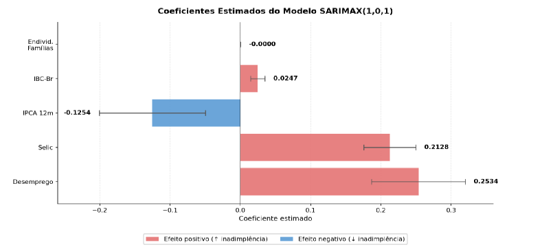
Figure 4 presents the estimated coefficients of the SARIMAX(1,0,1) model. All coefficients of the exogenous variables showed statistical significance at the 1% level, with the exception of household indebtedness (p = 0.165). Unemployment showed a positive coefficient of 0.2534 (p < 0.001), indicating that each additional percentage point in unemployment is associated with an increase of 0.25 percentage points in Nonpayment. The Selic rate also showed a significant positive effect (β = 0.2128; p < 0.001), with a magnitude similar to that of unemployment, highlighting the relevance of the credit cost transmission channel. The IBC-Br showed a positive coefficient of smaller magnitude (β = 0.0247; p < 0.001), suggesting that the expansion of credit volume in periods of higher activity may maintain pressure on Nonpayment.

Figure 4: Estimated Coefficients of the SARIMAX(1,0,1) Model.

Source: Own elaboration (Python/statsmodels and matplotlib, 2026).

The IPCA coefficient showed a negative sign (β = -0.1254; p = 0.001), which may seem counterintuitive. Three mechanisms can explain this finding: multicollinearity with the Selic, where the IPCA captures situations where inflation rises, but monetary policy has not yet reacted, potentially temporarily reducing default in real terms; the impact of inflation on real income may manifest at horizons longer than those captured by the contemporaneous specification; and the correlation structure between predictors, as observed in previous studies (Machado, 2025). This result reinforces that the IPCA should not be analyzed in isolation as a credit risk indicator, but in conjunction with monetary policy.

The AR(1) coefficient was 0.8965 (p < 0.001), indicating strong temporal persistence, where approximately 90% of the expected variation in a given month is already contained in the previous month’s value. The MA(1) coefficient was -0.0411 (p = 0.678), statistically not significant, but its inclusion in the model was supported by the comparison of information criteria, with the ARIMA(1,0,1) specification presenting an AIC of 6.03 and a BIC of 30.73, values lower than those obtained by the pure AR(1) specification. The presence of the MA component captures potential short-term shocks in the residuals, making the specification more robust in scenarios of point volatility. Table 3 summarizes the model’s performance metrics.

Table 3. SARIMAX(1,0,1) Model Performance Metrics and Summary of Projections by Macroeconomic Scenario

Metric	Value
Observations	164
Sample	Jul/2012 – Feb/2026
AIC	6.03
BIC	30.73
Log-Likelihood	4.984
MAE (adjustment)	0.1808
RMSE (fit)	0.2443
MAPE (adjustment)	3.12%
Ljung-Box p	0.95 (no autocorr.)
Heterosc. p-value	0.06

Source: Own elaboration (Python/statsmodels, 2026).

Macroeconomic scenarios

After the estimation, three scenarios were defined for projecting nonpayment until December 2026: optimistic, base, and pessimistic. The base scenario was calibrated from the medians of the Central Bank of Brazil’s (BCB, 2026a) Focus Report. The optimistic and pessimistic scenarios were constructed as symmetric deviations from the base scenario, representing monetary easing trajectories and labor market convergence to historically favorable levels (optimistic scenario), and fiscal deterioration, inflationary persistence, and interest rate hikes (pessimistic scenario), in line with the methodology for constructing stress scenarios adopted in credit risk analyses (BCB, 2024). In all scenarios, variables were kept constant throughout the projection horizon, which constitutes a methodological simplification. Table 4 summarizes the assumptions for each scenario.

Table 4. Summary of Projections by Macroeconomic Scenario

Scenario	Unemployment	Selic	IPCA	Nonpayment Dec/26
Optimistic	4.5%	8.5%	3.5%	6.30%
Basis	6.0%	12.5%	5.0%	7.22%
Pessimist	9.0%	16.0%	7.0%	7.98%

Source: Own elaboration (Python/statsmodels, 2026).

Robustness analysis – comparison between model specifications

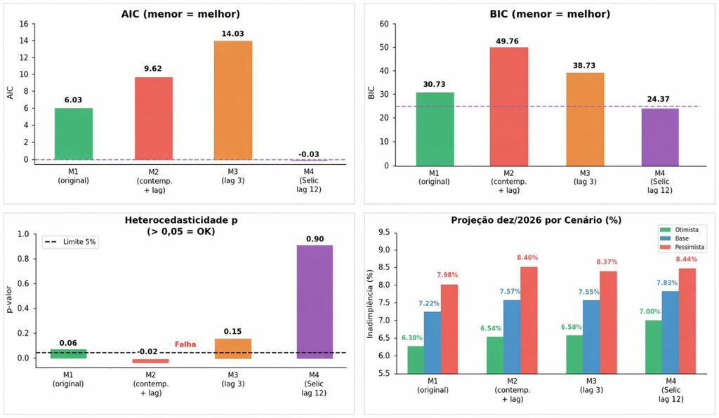
To assess the robustness of the adopted specification and verify whether the incorporation of lagged variables would improve predictive performance, four distinct specifications of the SARIMAX(1,0,1) model were tested. Model 1, adopted in this work, uses the five exogenous variables in their contemporary forms. Model 2 incorporates contemporary and lagged variables by three months. Model 3 replaces the contemporary variables with those lagged by three months. Model 4 replaces the contemporary Selic with the Selic lagged by twelve months, keeping the other variables contemporary.

Figure 5 and Table 5 present the comparison between the four specifications. The results revealed an important trade-off. Model 4 (Selic lag 12) presented the best information criteria (AIC = -0.03 versus 6.03 for Model 1, and BIC = 24.37 versus 30.73) and the best result in the homoscedasticity test (p = 0.90). However, its adoption would imply three disadvantages: loss of six observations in the sample (158 versus 164), loss of statistical significance of IPCA (p = 0.113), and divergence in projections (the base scenario went from 7.22% to 7.83% in December 2026). Models 2 and 3 presented inferior performance to Model 1 in all criteria, with Model 2 failing the homoscedasticity test (p = 0.02) and generating economically inconsistent coefficients. Given these results, the decision was made to maintain Model 1 for three objective reasons: a larger number of observations (164), a greater quantity of statistically significant coefficients, and more conservative scenario projections suitable for the objective of subsidizing the sizing of provisions. This analysis demonstrated that the choice of the original model was based on objective statistical and economic criteria.

Figure 5: Robustness Analysis — Comparison between Four SARIMAX(1,0,1) Specifications. Information criteria, residual diagnostics, scenario projections, and sample size.

Source: Own elaboration (Python/statsmodels, 2026).

Table 5. Robustness Analysis — Comparison between Four SARIMAX(1,0,1) Specifications

Criterion	M1 (initial)	M2	M3	M4 (“delay”12)
AIC	6.03	9.62	14.03	-0.03
BIC	30.73	49.76	38.73	24.37
Heterosc. p-value	0.06 (OK)	0.02 (Failure)	0.15 (OK)	0.90 (OK)
Ljung-Box p	0.95 (OK)	0.93 (OK)	0.97 (OK)	0.97 (OK)
Observations	164	164	164	158
Base scenario	7.22%	7.57%	7.55%	7.83%
IPCA signifies	p=0.001	p=0.000	p=0.000	p=0.113 (X)
Selected	YES	NO	NO	NO

Source: Own elaboration (Python/statsmodels, 2026).

Diagnosis of residuals and model validation

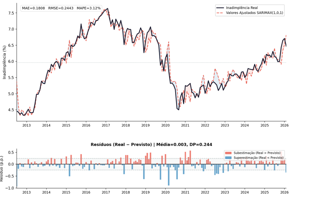
Figure 6 presents the comparison between the actual values and those fitted by the model, with the residuals in the lower panel. The model accurately tracks the trajectory of non-payment, with a MAPE of 3.12%, Mean Absolute Error (MAE) of 0.1808, and Root Mean Squared Error (RMSE) of 0.2443 percentage points in the fit to the historical series. The overlap between the line of observed values and the line of estimated values is almost complete throughout the entire period, with divergences visible only at specific moments of abrupt transition. The residuals oscillate around zero without exhibiting a systematic upward or downward trend, suggesting that the model is not persistently under- or overestimating non-payment. The performance metrics reported refer to the in-sample fit, calculated on the same dataset used for parameter estimation. This approach is defensible in short time series, provided it is accompanied by rigorous residual diagnostics (Hyndman and Athanasopoulos, 2021).

Figure 6: Actual Nonpayment vs. SARIMAX(1,0,1) Model Adjusted Values and Residual Analysis (bottom panel).

Source: Own elaboration (Python/statsmodels and matplotlib, 2026).

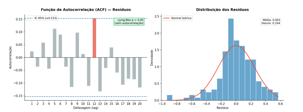
Figure 7 presents the formal diagnosis of the residuals. The ACF plot shows that no lag exceeds the 95% confidence interval limits (±0.153), confirming the absence of residual autocorrelation, a result consistent with the Ljung-Box test (p = 0.95). This characteristic indicates that the model has adequately captured the entire temporal structure of the series, and what remains in the residuals is random noise without an exploitable pattern. The histogram reveals an approximately normal distribution around zero, with a mean of 0.003 and a standard deviation of 0.244 percentage points, confirming the absence of systematic bias. The proximity to the normal distribution supports the statistical validity of the confidence intervals calculated for the coefficients and projections. The heteroscedasticity test resulted in p = 0.06, indicating homoscedasticity of the residuals at the 5% level. The set of these diagnostics validates the statistical adequacy of the model.

Figure 7: Diagnosis of SARIMAX(1,0,1) Model Residuals — Autocorrelation Function (ACF) and Distribution.

Source: Own elaboration (Python/statsmodels and matplotlib, 2026).

Scenario projection and practical implications

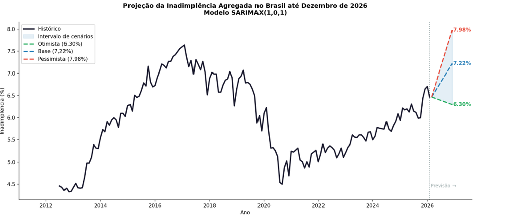
Figure 8 presents the projection of non-payment until December 2026. In the optimistic scenario, with unemployment falling to 4.5% and the Selic rate to 8.5%, non-payment converges to 6.30%. In the base scenario, with unemployment at 6.0% and Selic at 12.5%, it is projected at 7.22%. In the pessimistic scenario, with unemployment at 9.0% and Selic at 16.0%, non-payment may reach 7.98%. The graph combines the observed historical series with the three projected trajectories, each accompanied by a shaded band corresponding to the 95% confidence interval of the forecast. The progressive widening of the range between scenarios over the projection horizon highlights how small differences in initial macroeconomic assumptions amplify into material divergences in projected non-payment levels, given the persistent nature of the indicator captured by the AR(1) coefficient. This graphical representation is useful for risk analysts, as it makes the sensitivity of the outcome to the adopted hypotheses visible and allows for the sizing of the uncertainty interval associated with each provisioning decision.

Figure 8: Projection of Aggregate Non-payment in Brazil until December 2026 under Three Macroeconomic Scenarios.

Source: Own elaboration (Python/statsmodels and matplotlib, 2026).

The amplitude of 1.68 percentage points between the extreme scenarios has practical implications. Considering a total credit balance of the Brazilian financial system close to R$ 6 trillion in 2025, this difference represents an additional exposure of approximately R$ 100 billion in the pessimistic scenario compared to the optimistic one, a magnitude that directly affects the level of provisions required by regulatory standards. The sensitivity of nonpayment to the Selic (β = 0.2128) indicates that each 1 percentage point increase cycle in the benchmark rate is associated with a 0.21 percentage point increase in aggregate nonpayment, highlighting the importance of monitoring Copom’s decisions in the credit risk management of institutions. An important limitation is that the scenarios assume constant values for exogenous variables throughout the horizon, disregarding the temporal dynamics of macroeconomic variables themselves.

The aggregate non-payment in the financial system is an indicator directly connected to the operational health of banking institutions. The results indicate that when non-payment rises, the financial result deteriorates due to the need for the constitution of additional provisions, the provision coverage ratio is pressured, potentially demanding capital injections, and the origination of new credit tends to be restricted. The projections of this work indicate that, in the pessimistic scenario, non-payment may reach 7.98% in December 2026, a level not observed since the recessionary period of 2015–2016. For banks, this suggests that the credit cycle tends to become more conservative, with higher spreads and more restrictive granting criteria, especially in segments more sensitive to income.

From the perspective of credit risk management, the projections of this model offer a quantitative input to calibrate the systemic risk parameters used in the institutions’ internal models. The estimated AR(1) coefficient = 0.8965 indicates that default is highly persistent, implying that once a cycle of increase begins, the reversion to the historical average takes time. The findings suggest two important points for risk areas: first, probability of default models that only incorporate current default as a macroeconomic covariate may underestimate the risk in periods of cycle acceleration; second, collection and credit recovery strategies need to be anticipated in relation to the deterioration of aggregate indices. The sensitivity to unemployment (β = 0.2534) also reinforces the need for continuous monitoring of the labor market as a leading indicator of credit risk in retail portfolios.

The sizing of provisions for expected losses is one of the most direct applications of the results of this work. The projected range between scenarios — 1.68 percentage points between the optimistic (6.30%) and the pessimistic (7.98%) in December 2026 — represents, on a credit balance of R$ 6 trillion, a difference of approximately R$ 100 billion in defaulted exposure. For an institution with a credit portfolio of R$ 10 billion, the same proportional difference implies a variation of R$ 168 million in the calculation base for provisions, which can represent a material impact on the fiscal year’s results. Scenario models like the one developed in this work allow financial planning and control areas to simulate the need for additional provisions in each scenario and incorporate this uncertainty into the annual budgeting process. This approach is especially relevant from the perspective of CMN Resolution No. 4.966/2021, which requires prospective consideration of multiple economic scenarios in the measurement of expected credit losses.

From a regulatory standpoint, the results of this work dialogue directly with two pillars of the current normative framework. CMN Resolution No. 4.557/2017 determines that the credit risk management structure must consider the current macroeconomic environment and its short-term projections, a requirement that the SARIMAX model meets by translating variables such as Selic, unemployment, and economic activity into quantitative default forecasts. CMN Resolution No. 4.966/2021, in turn, introduced the requirement for a forward-looking approach in the measurement of expected losses, with consideration of multiple plausible scenarios, a structure exactly replicated by the optimistic, base, and pessimistic scenario methodology adopted in this work. Furthermore, the interpretability of the SARIMAX model, where each coefficient has direct economic meaning, is a relevant differential in contexts of banking audit and supervision, where black-box models face increasing restrictions on their use for capital adequacy purposes.

The study results indicate that continuous monitoring of the Selic rate and the unemployment rate is important for the credit risk management of financial institutions. Following the minutes of the Copom meetings and the Focus Bulletin projections can serve as early warning signs of pressure on future defaults, given the lagged effect of the Selic rate (up to 12 months). Regarding unemployment, monthly monitoring of the PNAD Contínua and Caged data are immediate alert indicators, as the effect on defaults is contemporaneous. Periodic updating of the model with new data, ideally monthly, following the release of the series by the BCB and IBGE, is fundamental to preserving the predictive relevance of the projections over time.

For the budgeting and provisioning sizing process, the use of the base scenario as a central reference is indicated for financial planning, with the optimistic and pessimistic scenarios serving as the lower and upper limits of the sensitivity range. The range of 6.30% to 7.98% projected for December 2026 can be incorporated into credit portfolio stress testing exercises, allowing for the sizing of incremental capital needs under adverse conditions. Additionally, macroeconomic scenarios can be reviewed quarterly, incorporating the projections from the Focus Report and the guidelines from the Monetary Policy Committee (Copom), to keep the assumptions updated with the current economic context.

For the purpose of compliance with CMN Resolutions No. 4.557/2017 and 4.966/2021, the SARIMAX methodology with macroeconomic scenarios can be formally documented as a component of the institution’s credit risk management framework. The documentation may include: a description of the variables used and their sources; model selection criteria and robustness analysis comparing alternative specifications; update frequency and parameter review; and a periodic backtesting procedure to validate predictive accuracy. The model may be submitted for independent validation by the model validation area before its application for capital adequacy purposes, ensuring compliance with the good model governance practices established by the Central Bank of Brazil.

In summary, the study demonstrated the capacity of the SARIMAX(1,0,1) model to predict aggregate default in the Brazilian financial system, identifying unemployment and the Selic rate as main determinants with different transmission speeds. The robustness analysis confirmed the adequacy of the contemporary model specification, and the residual diagnostics validated its statistical accuracy. Projections under optimistic, base, and pessimistic scenarios revealed a significant range of uncertainty, with direct implications for provisioning and credit risk management, aligning with regulatory requirements for a prospective approach.

4. Conclusion

The present study sought to model and predict the aggregate non-payment of the Brazilian financial system using the SARIMAX(1,0,1) model with contemporary exogenous macroeconomic variables, projecting its trajectory until December 2026 under optimistic, base, and pessimistic scenarios, with the aim of supporting risk analyses and provisioning sizing. It was found that aggregate non-payment is strongly determined by unemployment and the Selic rate, which act with distinct transmission speeds. Unemployment demonstrated a predominantly contemporary effect, while the Selic exhibited an increasing correlation with non-payment in lags of up to twelve months, reflecting the gradual transmission mechanism of credit cost. A strong temporal persistence in the indicator was also identified, captured by the AR(1) coefficient of 0.8965. The model specification was validated by information criteria and coefficient stability, and the residual diagnostics confirmed its statistical adequacy, with a Mean Absolute Percentage Error (MAPE) of 3.12%. The projections indicated that non-payment could range between 6.30% and 7.98% in December 2026, revealing a range of 1.68 percentage points between the extreme scenarios.

This projected range has direct implications for credit risk management and the sizing of provisions in financial institutions, offering a quantitative input aligned with the regulatory requirements of CMN Resolutions No. 4.557/2017 and 4.966/2021, which demand a prospective approach and the consideration of multiple scenarios. The interpretability of the SARIMAX model constitutes a differential in contexts of banking audit and supervision. However, the study presents limitations, such as the assumption of constant values for exogenous variables throughout the projection horizon, the absence of formal treatment of structural breaks, and the restriction to linear relationships. For future studies, it is suggested to explore hybrid models that combine SARIMAX with neural networks, the incorporation of dynamic projections of macroeconomic variables, and the investigation of explainability techniques (XAI) to enhance model transparency in regulatory contexts.

Bibliographic References

BANCO CENTRAL DO BRASIL. Focus – Relatório de Mercado. Brasília: BCB, 28 mar. 2026. Disponível em: https://www.bcb.gov.br/publicacoes/focus. Acesso em: mar. 2026.

BANCO CENTRAL DO BRASIL. Relatório de Estabilidade Financeira. Brasília: BCB, 2024. Disponível em: https://www.bcb.gov.br. Acesso em: abr. 2026.

BARBOSA, J. H. F. Prociclicidade do risco de crédito: um modelo point in time para o risco da carteira de crédito agregada dos bancos brasileiros. 2007. Dissertação (Mestrado em Administração) — Universidade Federal do Paraná, Curitiba, 2007.

Basel COMMITTEE ON BANKING SUPERVISION. Guidelines: Guidance on credit risk and accounting for expected credit losses. Basel: BIS, 2015. Disponível em: https://www.bis.org/bcbs/publ/d350.htm. Acesso em: abr. 2026.

BCB/SGS, 2026 [Referência completa não encontrada no documento original]

BELLOTTI, T.; CROOK, J. Support vector machines for credit scoring and discovery of significant features. Expert Systems with Applications, v. 36, n. 2, p. 3302–3308, 2009.

BERNANKE, B. S.; GERTLER, M. Agency costs, net worth, and business fluctuations. American Economic Review, v. 79, n. 1, p. 14–31, 1989.

BOUDOUKH, J.; RICHARDSON, M.; WHITELAW, R. F. “Out-of-Sample” Equity Premium Prediction: Combination Forecasts and Links to the Real Economy. The Review of Financial Studies, v. 23, n. 2, p. 821–862, 2009.

BRASIL. Conselho Monetário Nacional. Resolução n.º 4.557, de 23 de fevereiro de 2017. Dispõe sobre a estrutura de gerenciamento de riscos e a estrutura de gerenciamento de capital. Brasília: Banco Central do Brasil, 2017. Disponível em: https://www.bcb.gov.br. Acesso em: abr. 2026.

BRASIL. Conselho Monetário Nacional. Resolução n.º 4.966, de 25 de novembro de 2021. Dispõe sobre a mensuração de perdas esperadas associadas ao risco de crédito. Brasília: Banco Central do Brasil, 2021. Disponível em: https://www.bcb.gov.br. Acesso em: abr. 2026.

ENDERS, W. Applied econometric time series. 4. ed. Hoboken: Wiley, 2015.

GUJARATI, D. N.; PORTER, D. C. Econometria básica. 5. ed. Porto Alegre: AMGH, 2011.

HYNDMAN, R. J.; ATHANASOPOULOS, G. Forecasting: Principles and Practice. 3. ed. Melbourne: OTexts, 2021. Disponível em: https://otexts.com/fpp3/. Acesso em: mar. 2026.

IBGE/PNAD Contínua, 2026 [Referência completa não encontrada no documento original]

JIMÉNEZ, G. et al. Credit supply: Identifying balance-sheet channels with loan applications and granted loans. American Economic Review, v. 102, n. 5, p. 2301–2326, 2008.

MACHADO, A. R. Modelagem e previsão da taxa de inadimplência: uma análise comparativa de modelos ARIMA, redes neurais e abordagens híbridas, sem e com variáveis exógenas. 2025. Dissertação (Mestrado em Economia) — Escola de Políticas Públicas e Governo, Fundação Getulio Vargas, Brasília, 2025

MISHKIN, F. S. The economics of money, banking, and financial markets. 11. ed. New York: Pearson, 2016.

Python/matplotlib, 2026 [Referência completa não encontrada no documento original]

Python/pandas, 2026 [Referência completa não encontrada no documento original]

Python/statsmodels e matplotlib, 2026 [Referência completa não encontrada no documento original]

Python/statsmodels, 2026 [Referência completa não encontrada no documento original]

THOMAS, L. C.; CROOK, J.; EDELMAN, D. Credit scoring and its applications. 2. ed. Philadelphia: SIAM, 2017.

Article originating from the Final Course Work of the Specialization in Data Science and Analytics of the MBA USP/Esalq

To learn more about the course, click here and access the MBX Academy platform