Accuracy of Demand Forecasting Models in the Brazilian Soybean Market

Votdk, Jonwfer Lauro; Ribeiro, Rodolfo

doi:10.22167/2675-6528-202602240

Article

September 15, 2026

Accuracy of Demand Forecasting Models in the Brazilian Soybean Market

Jonwfer Lauro Votdk; Rodolfo Ribeiro

DOI: 10.22167/2675-6528-202602240

Article derived from a Final Course Work (TCC), with content based on the student’s original work and adapted to the editorial format of the E&S Magazine with the support of the ResumeAI tool, an artificial intelligence solution developed by the Pecege Institute for textual synthesis and organization.

Abstract

Demand forecasting is a critical component for planning and risk management decisions in commodity chains, such as soybeans, where seasonality and volume concentration can amplify operational and economic impacts. The accuracy of forecasting models applied to the monthly export volume of Brazilian soybeans was evaluated, with the objective of identifying the forecasting model with the best performance for this context and estimating the economic exposure associated with forecasting error. Monthly data from January 2016 to December 2025 were used, obtained from Comex Stat for HS code 12019000. The data were segregated into an estimation sample (2016–2024) and a test sample (2025) for out-of-sample validation. Five methods were implemented: Naive, Seasonal Naive, 3-month moving average, 12-month moving average, and Seasonal Exponential Smoothing (ETS). Performance was measured by MAE, RMSE, MAPE, WMAPE, and BIAS, with WMAPE adopted as the primary criterion for weighting the error by the realized volume; additionally, the cost of error was estimated in US$ based on the monthly FOB value. The results indicated that ETS showed the best overall performance in the test sample, with lower error and bias, followed by Seasonal Naive, while Naive and moving averages showed greater underestimation, especially in peak months. The explicit incorporation of seasonality and the use of complementary metrics reduced uncertainty and economic exposure associated with forecasting error in the analyzed scenario.

Keywords: Error cost; Demand planning; Seasonality; Exponential smoothing; WMAPE.

1. Introduction

Brazilian agribusiness has soy as a fundamental pillar, positioning it centrally in international trade of agricultural commodities. The oilseed accounts for approximately half of the volume of grains produced in the country (Agência GOV, 2025). Brazil stands out as the world’s largest producer, with an estimated production of 169.49 million tons in the 2024/2025 harvest, cultivated in about 58% of the national agricultural area, which corresponds to approximately 47.61 million hectares (Brasil, 2025). This projection underscores the economic, logistical, and strategic relevance of the sector for the trade balance and for the supply of essential production chains, such as animal feed, vegetable oil, and biofuels (EMBRAPA, 2025). Furthermore, soy has a significant participation in both the external market and domestic consumption, with expressive volumes of export and processing (Vieira Filho, 2024).

The importance of soybeans in Brazil transcends primary production, extending through a complex value chain that includes planting decisions, storage, crushing, transportation, commercialization, and export. All these stages are highly sensitive to fluctuations in demand, prices, exchange rates, climatic conditions, and infrastructure (SCOT Consultoria, 2025). In 2024, the volume of soybeans in grains exported reached 98.815 million tons, while 55.811 million tons were destined for domestic consumption. This scenario highlights the magnitude of the chain and the need for effective coordination between supply and demand. Consequently, demand forecasting becomes a crucial element for companies and agents involved in sales and operations planning, supply, origination, and inventory management (EMBRAPA, 2025).

Despite its relevance, soybean market demand forecasting presents inherent challenges, given that the time series is influenced by structural and cyclical factors. Previous studies on soybeans in Brazil indicate that statistical models, such as exponential smoothing, regression, and ARIMA, can generate useful results, but their performance varies according to the series’ characteristics, seasonality, forecasting horizon, and the occurrence of external shocks (Schmidt et al., 2019). In the field of demand forecasting, there is a consensus that no universally superior method exists for all contexts, which makes comparing different models an indispensable step to identify the most suitable approach for the segment studied (Makridakis and Hibon, 2000). The literature also warns that accuracy evaluation is complex, as different metrics can lead to distinct rankings among models and, in certain situations, may present practical problems or misleading interpretations (Hyndman and Koehler, 2006). Therefore, comparison with reference models, or benchmarks, is fundamental, as sophisticated forecasts do not always outperform simpler methods (Goodwin, Petropoulos and Hyndman, 2017).

More accurate forecasts are essential in the business environment, especially in sales and operations planning (S&OP) operations, as they contribute to the reduction of stockouts, excess inventory, misalignments between supply and demand, and the waste of working capital. Accuracy should not be seen merely as the proximity between the forecasted and actual values, but also as the absence of bias, stability over time, and adequacy to the observed horizon. Thus, the comparative analysis between forecasting models in the Brazilian soybean market is relevant from both an academic and managerial perspective, offering subsidies for planning, supply, and commercialization decisions (Hyndman and Athanasopoulos, 2021). Given this context, the objective of this study is to identify the forecasting model with the best performance for this context and to estimate the economic exposure associated with forecasting error.

2. Material and Methods

This study was characterized as an applied research, with a quantitative approach and a descriptive-comparative objective, evaluating the performance of different models for forecasting external demand for Brazilian soybeans from the comparison of accuracy metrics. The analysis was based on monthly time series of soybean grain exports.

The data were extracted from Comex Stat, the official system of the Ministry of Development, Industry, Trade and Services (MDIC) for foreign trade statistics, using NCM code 12019000 (Soybeans, whether or not crushed, other than for sowing). The analyzed period comprised January 2016 to December 2025, totaling 120 monthly observations. The sample was divided into two subsets: January 2016 to December 2024 for model estimation, and January to December 2025 for validation. The query in Comex Stat can be accessed at: https://comexstat.mdic.gov.br/pt/geral/149927.

The variables used were treated and are detailed in Table 1.

Table 1. Variables Used

Variables	Description
Type	Diferentiation between Test Sample and Estimation Sample
Year	Year referring to the presented data
Month	Reference month for the presented data
Date	Complete data referring to the presented data
NCM Code	Mercosur Common Nomenclature
NCM Description	Description of the Southern Common Market Nomenclature
Net Kilogram	Volume extracted from Comex Stat in kg
Volume in tons	Volume converted to tons
FOB Value USD$	FOB (“Free On Board”) value in dollars

Source: Original survey data

The validation strategy adopted was out-of-sample validation, ensuring that the realized values for 2025 were not used in the model construction phase. The predictions generated by each model, as well as the calculation of error metrics, were implemented using Excel formulas in an auxiliary spreadsheet, guaranteeing traceability between original data, predictions, and evaluation results. The models were estimated with data from the estimation sample and used to generate predictions for the 12 months of 2025, compared with the realized values in that period to evaluate the predictive capacity of each method.

Five forecasting models were implemented:

The Naive Model assumes that the best forecast for a period corresponds to the value observed in the immediately preceding period. The value of December 2024 was considered for January 2025, and subsequent forecasts kept this value fixed. This model was used as a “benchmark”.
The Seasonal Naive Model considered annual seasonality, assigning as a forecast for a month the value observed in the same month of the previous year (e.g., January 2025 was the actual value from January 2024). This model is suitable for monthly series with recurring seasonal patterns.
The 3-month moving average was implemented from the arithmetic mean of the three immediately preceding months. For out-of-sample validation, an auxiliary series was created to use the model’s own predictions generated in the test sample months.
The 12-month moving average was estimated analogously, considering 12 periods to capture long-term patterns of the series. An auxiliary series was also created to consider the forecast data of this model for the months of 2025.
The Exponential Smoothing (ETS) Model with error, trend, and seasonality was implemented through the Excel formula FORECAST.ETS(), which automatically estimates the series components based on historical data. The period from January 2016 to December 2024 and a 12-month seasonality were considered.

The performance of the models was evaluated by error and bias metrics, calculated in Excel from the comparison between predicted and actual values of the test sample. The metrics used were:

Mean Absolute Error (MAE): Calculated by equation (1): MAE = (1/n) × Σ|Yт – Ўт| where: n is the number of calculated months, equal to 12; Yт is the realized volume per month in 2025; and Ўт is the volume observed by the model in the comparison month.
Root Mean Square Error (RMSE): Calculated by equation (2): RMSE = √(1/n) × Σ(Yт – Ўт)² where: n is the number of months calculated, equal to 12; Yт is the volume achieved per month in 2025; and Ўт is the volume observed by the model in the comparison month.
Mean Absolute Percentage Error (MAPE): Calculated by equation (3): MAPE = (100/n) × Σ|(Yт – Ўт) / Yт| where: n is the number of months calculated, equal to 12; Yт is the realized volume per month in 2025; and Ўт is the volume observed by the model in the comparison month.
Weighted Mean Absolute Percentage Error (WMAPE): Calculated by equation (4): WMAPE = (Σ|Yт – Ўт| / ΣYт) × 100 where: Yт is the realized volume per month in 2025; and Ўт is the volume observed by the model in the comparison month.
BIAS (bias): Calculated by equation (5): BIAS = (1/n) × Σ(Ўт – Yт) where: n is the number of calculated months, equal to 12; Yт is the volume realized per month in 2025; and Ўт is the volume observed by the model in the comparison month.

Beyond statistical metrics, the economic impact of demand forecast error was estimated using the FOB value US$ extracted from Comex Stat for NCM 12019000 and the test sample. The objective was to understand the financial impact of the error, representing the value associated with the incorrectly forecasted volume. The unit price per ton for each month of 2025 was calculated by equation (6):

PUT = FOB Value US$т / Yт

where: PUT is the monthly unit price per ton; FOB value US$t is the observed value in month t; and Yt is the volume observed in the comparison month.

Next, the monthly error volume for each prediction model was obtained by equation (7):

et = Yt – Yt

where: eт is the error in the month; Ўт is the volume observed by the model in the comparison month; and Yт is the volume realized per month.

When et was less than 0, the forecast was considered underestimated; when et was greater than 0, the forecast was considered overestimated. The cost of the error was estimated as the economic exposure linked to the unit price of the analysis month, according to equation (8):

Ct = |et| × PUT

where: Cт is the cost of error; eт is the error in the month; and PUT is the monthly unit price per ton.

In summary, the forecasting models were calculated on the test sample for the 12 months of 2025, ensuring comparability. Predictive performance was measured by complementary error and bias metrics (MAE, RMSE, MAPE, WMAPE, and BIAS), calculated from the comparison between predicted and actual values, and by the cost of error. For the selection of the best-performing model, WMAPE was adopted as the main criterion, as it represents the percentage error weighted by the actual volume, reducing distortions in periods of low magnitude and facilitating managerial interpretation. MAE and RMSE were used to identify the magnitude of the error in tons, and BIAS to identify the tendency of overestimation or underestimation. The cost of error in US$ provided an economic dimension of demand underestimation and overestimation.

3. Results and Discussion

This study evaluated the accuracy of different demand forecasting models applied to the monthly export volume of soybeans in Brazil, comparing the forecasts generated from the estimation sample with the actual values in the test sample. The models’ performance was measured by complementary error and bias metrics, such as Mean Absolute Error (MAE), Root Mean Squared Error (RMSE), Mean Absolute Percentage Error (MAPE), Weighted Mean Absolute Percentage Error (WMAPE), and BIAS, in addition to exposure to the cost of error. WMAPE was adopted as the main selection criterion, as it reflects the percentage error weighted by the actual volume, aligning with the managerial impact of the error. The other metrics provided interpretive support, with MAE and RMSE evaluating the magnitude of the error, MAPE as an additional percentage measure, and BIAS identifying the systematic tendency of overestimation or underestimation (Hyndman and Koehler, 2006).

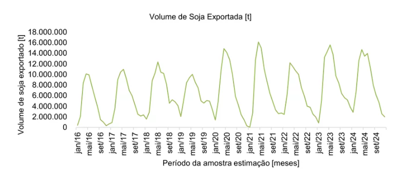
In the estimation sample, from January 2016 to December 2024, a seasonal behavior was observed in the volume of soybeans exported, impacted by the cultivation cycle. Figure 1 illustrates this pattern, with low volumes at the beginning of the year, peaks between March and May, and a gradual reduction in the second half of the year. This seasonality reinforces the need for models that consider these variations (Hyndman and Athanasopoulos, 2021).

Figure 1. Volume of Soy exported in tons between January/2016 and December/2024

Source: Original research results and data extracted from the Comex Stat system (MDIC)(Brazil, [n.d.])

The demand forecasts for the months of 2025, generated by the Naive, Seasonal Naive, 3-month Moving Average (MA3), 12-month Moving Average (MA12), and Seasonal Exponential Smoothing (ETS) models, were calculated from the estimation sample data. Table 2 presents these predicted values in comparison with the realized volume.

Table 2. Demand forecast by the chosen models for the months of 2025

Date	Performed	Ingenuous	Seasonal naive	MM3	MM12	ETS
Jan/25	1.069.087	2.006.054	2.854.860	3.089.530	8.233.987	3.114.695
Feb/25	6.428.317	2.006.054	6.608.134	2.549.461	8.682.248	6.473.643
Mar/25	14.657.781	2.006.054	12.600.297	2.548.348	8.855.090	13.037.785
Apr/25	15.271.914	2.006.054	14.687.842	2.729.113	8.542.990	14.641.939
may/25	14.099.745	2.006.054	13.436.721	2.608.974	8.030.919	14.481.086
Jun/25	13.420.319	2.006.054	13.959.612	2.628.812	7.580.435	13.257.230
July/25	12.257.306	2.006.054	11.249.768	2.655.633	7.048.837	10.679.878
Aug/25	9.325.162	2.006.054	8.037.754	2.631.140	6.698.760	8.399.443
Sep/25	7.339.951	2.006.054	6.104.265	2.638.528	6.587.177	6.477.453
Oct/25	6.727.671	2.006.054	4.709.739	2.641.767	6.627.419	5.584.987
Nov/25	4.197.159	2.006.054	2.552.798	2.637.145	6.787.226	4.543.391
12/25	3.383.155	2.006.054	2.006.054	2.639.147	7.140.095	3.861.693

Source: Original research results and data extracted from the Comex Stat system (MDIC)(Brazil, [n.d.])

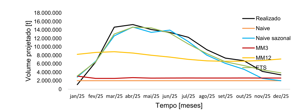
The comparison between the realized volume and the forecasts of each model for 2025, presented in Figure 2, revealed that the Naive seasonal and ETS models were the closest to the actual volume. Both models consider seasonality as a forecasting factor. The ETS, by considering the 12-month seasonality and using 9 years of data, managed to identify recurrence and trend. The Naive seasonal replicated the 2024 pattern, showing peaks and troughs consistent with soybean export demand. This performance is consistent with studies indicating that simple methods can be competitive when they capture seasonality (Makridakis and Hibon, 2000).

Figure 2. Comparison between the volume achieved and the forecasts of each model for soybeans exported in 2025

Source: Original research results and data extracted from the Comex Stat system (MDIC)(Brazil, [n.d.])

In contrast, the Naive, MM3, and MM12 models did not approach the volume realized in 2025. The Naive model, based solely on the previous month, significantly underestimated the volume, as it considered the low volume of December 2024 for all 2025 forecasts. The MM3 presented a similar result, influenced by the low volumes from October to December 2024 and using its own forecasts for subsequent months. The MM12 captured seasonality but with reduced amplitude and horizontal displacement, which is due to the inclusion of average values calculated by the model itself in the peak months, resulting in lower forecasts than realized (Hyndman and Athanasopoulos, 2021; Makridakis and Hibon, 2000).

The analysis of error metrics for the test sample period, classified by WMAPE, confirmed the models’ performance. Table 3 details these results.

Table 3. Demand forecasting model metrics

Model	MAE [t]	RMSE [t]	MAPE [%]	WMAPE [%]	BIAS [t]
ETS	851.536	1.045.768	23,8%	9,4%	-302.029
Seasonal naive	1.198.291	1.335.352	28,8%	13,3%	-780.810
MM12	4.047.505	4.670.175	94,2%	45,2%	-1.446.865
MM3	6.685.071	7.907.642	75,8%	74,2%	-6.348.331
Ingenuous	7.164.904	8.411.923	74,9%	79,5%	-7.008.743

Source: Original research results

The ETS model presented the lowest MAE (851.536 t) and RMSE (1,045,768 t), indicating the greatest average proximity between forecast and actual values and the ability to avoid large divergences. The seasonal Naive model was the second best in both criteria (MAE of 1,198,291 t and RMSE of 1,335,352 t), which is expected for a model that captures annual seasonality. The Naive and MM3 models registered significantly higher MAE and RMSE, suggesting that their forecasts were far from the actual values, especially in peak months (Hyndman and Athanasopoulos, 2021).

Regarding MAPE, ETS obtained the lowest value (23.8%), followed by Seasonal Naive (28.8%). The MM12 MAPE was high (94.2%), influenced by months with low actual volume, such as January, where the percentage error was 670.2%. This sensitivity of MAPE to low volumes highlights the importance of evaluating it in conjunction with other metrics (Hyndman and Koehler, 2006).

The WMAPE, the main criterion, confirmed ETS as the best model (9.4%), followed by Seasonal Naive (13.3%). The MM12 (45.2%), MM3 (74.2%), and Naive (79.5%) models showed considerably higher WMAPEs. Models without the capacity to capture seasonality, such as Naive and MM3, underestimated the peaks of the first half of the year, concentrating absolute errors in higher realized volumes and, consequently, increasing the WMAPE.

The BIAS, which indicates the direction of the error, showed a predominant tendency of underestimation in all models. The ETS registered the bias closest to zero (-302.029 t), while the seasonal Naive (-780.810 t) also underestimated, but to a lesser extent than the others. The Naive (-7.008.743 t) and MM3 (-6.348.331 t) models exhibited the largest negative biases, indicating a continuous underestimation that can lead to conservative decisions and demand underestimation (Hyndman and Athanasopoulos, 2021).

To complement the statistical metrics, the cost of the error was calculated in dollars, considering the monthly FOB Value US$ and the exported volume in each month of 2025. Table 4 presents the monthly unit cost per ton.

Table 4. Monthly unit cost in dollars per ton

Date	Volume in tons	US$ FOB Value	Unit cost
Jan/25	1.069.087	$ 433.412.725	$ 405,40
Feb/25	6.428.317	$2.543.652.430	$ 395,69
Mar/25	14.657.781	$5.673.615.141	$ 387,07
Apr/25	15.271.914	$5.864.208.310	$ 383,99
may/25	14.099.745	$5.501.158.133	$ 390,16
Jun/25	13.420.319	$5.337.449.698	$ 397,71
July/25	12.257.306	$ 5.001.850.667	$ 408,07
Aug/25	9.325.162	$3.868.955.860	$ 414,89
Sep/25	7.339.951	$3.103.031.251	$ 422,76
Oct/25	6.727.671	$2.878.022.046	$ 427,79
Nov/25	4.197.159	$1.827.759.344	$ 435,48
12/25	3.383.155	$ 1.498.479.236	$ 442,92

Source: Original research results and data extracted from the Comex Stat system (MDIC)(Brazil, [n.d.])

The variation in unit price throughout 2025, with lower prices in higher volume months and higher prices in lower volume months, indicates that the economic impact of the forecast error is influenced by both unit price and volume. The annual cost of the error for each model was calculated and is detailed in Table 5.

Table 5. Cost of error for each demand forecasting model

Prediction model	Cost underestimation	Cost overestimation	Total cost
Ingenuous	$34.057.820.976	$379.850.481	$34.437.671.457
Seasonal naive	$4.936.315.383	$1.009.597.624	$5.945.913.007
MM3	$31.253.339.787	$819.096.726	$32.072.436.513
MM12	$13.096.524.451	$6.588.500.089	$19.685.024.540
ETS	$2.815.053.787	$1.358.749.449	$4.173.803.236

Source: Original research results and data extracted from the Comex Stat system (MDIC)(Brazil, [n.d.])

The largest portion of the error cost for all evaluated models is linked to underestimation, which is consistent with the observed negative biases. This underestimation represents a significant operational risk, potentially generating logistical constraints and lower readiness to meet demand during export peaks (Hyndman and Athanasopoulos, 2021; Fildes, Ma and Kolassa, 2019).

In this context, ETS presented the lowest exposure to the total cost of error, with $4,173,803,236, which corresponds to approximately 9.5% of the value exported in 2025. This value was significantly lower than the error costs of the other models. Seasonal Naive registered $5,945,913,007, while models that did not capture seasonality, such as MM12 ($19,685,024,540), MM3 ($32,072,436,513), and Naive ($34,437,671,457), presented much higher error costs. This difference demonstrates that the ETS and Seasonal Naive models not only outperformed the others in accuracy but were also more effective in reducing the economic exposure associated with forecasting error.

In summary, the statistical and cost metrics converged to the same practical conclusion: the ETS model was consistently superior. It led in the WMAPE criterion and presented the lowest MAE and RMSE, the lowest MAPE, the BIAS closest to zero, and the lowest error cost. The seasonal Naive, although not the best, demonstrated good performance and can serve as a useful benchmark for monitoring the added value of more sophisticated models (Goodwin, Petropoulos, and Hyndman, 2017). On the other hand, the moving average models and the Naive did not prove adequate for the dynamics of 2025, failing to capture seasonality and resulting in significantly higher errors (Makridakis and Hibon, 2000).

4. Conclusion

This study evaluated the accuracy of different forecasting models applied to Brazil’s monthly soybean grain export volume, seeking to identify the best-performing model and estimate the economic exposure associated with forecasting error. It was found that the Seasonal Exponential Smoothing (ETS) model consistently showed the best performance in the test sample, with lower weighted mean absolute percentage error (WMAPE), lower absolute error (MAE and RMSE), and lower bias (BIAS). The seasonal Naive model also demonstrated good performance, positioning itself as a robust comparative benchmark. In contrast, the Naive, 3-month Moving Average, and 12-month Moving Average models failed to capture the intrinsic seasonality of the time series, resulting in significant underestimation of export volumes, especially during peak months, and consequently, substantially higher errors and greater economic exposure.

The study’s main contribution lies in identifying a forecasting approach that minimizes uncertainty and economic exposure in the planning of the Brazilian soybean export chain. The adoption of the ETS model, which explicitly incorporates seasonality, offers managerial subsidies for more accurate decisions in sales and operations planning, supply, and risk management. The analysis of the cost of error in dollars revealed that demand underestimation represents the largest share of economic exposure, indicating significant operational risks, such as logistical constraints and lower preparedness to meet demand. The joint evaluation of error and bias metrics, complemented by the quantification of economic impact, proved essential for a comprehensive understanding of model performance, reinforcing that the analysis of a single metric can lead to misleading interpretations.

Bibliographic References

Agência GOV. Conab: safra de grãos 2024/25 será recorde com destaque para milho e soja. Agência Gov, 14 ago. 2025. Disponível em: . Acesso em: 10 abril 2026.

Brasil. Ministério do Desenvolvimento, Indústria, Comércio e Serviços (MDIC). Comex Stat: consulta geral (ID 149927). Brasília, DF: MDIC, [s.d.]. Disponível em: https://comexstat.mdic.gov.br/pt/geral/149927. Acesso em: 10 abril 2026.

Brasil. Secretaria de Comunicação Social da Presidência da República. Produção de grãos deve bater recorde com 332,9 milhões de toneladas na safra 2024/25. Gov.br, 15 maio 2025. Disponível em: . Acesso em: 10 abril 2026.

EMBRAPA. Dados econômicos. Londrina: Embrapa Soja, 2025. Disponível em: . Acesso em: 10 abril 2026.

Fildes, R.; Ma, S.; Kolassa, S. Retail forecasting: Research and practice. International Journal of Forecasting, v. 35, n. 1, p. 1–22, 2019. DOI: 10.1016/j.ijforecast.2018.06.004.

Goodwin, P.; Petropoulos, F.; Hyndman, R. A note on upper bounds for forecast-value-added relative to naïve forecasts. Journal of the Operational Research Society, v. 68, n. 9, p. 1082-1084, 2017.

Hyndman, R.; Athanasopoulos, G. Forecasting: Principles and Practice. 3. ed. OTexts, 2021. Disponível em: https://otexts.com/fpp3/.

Hyndman, R.; Koehler, A. Another look at measures of forecast accuracy. International Journal of Forecasting, v. 22, n. 4, p. 679–688, 2006.

Makridakis, S.; Hibon, M. The M3-Competition: results, conclusions and implications. International Journal of Forecasting, v. 16, n. 4, p. 451–476, 2000.

Schmidt, C.; Tayano, P; Santos, J.; Marujo, L.; Proença, G. Previsões estatísticas com base em séries temporais da cultura da soja no Brasil. Revista Técnico-Científica do CREA-PR, 2020.

SCOT Consultoria. Carta Grãos e Agricultura – Conab confirma produção histórica de soja no Brasil. Scot Consultoria, 27 maio 2025. Disponível em: . Acesso em: 10 abril 2026.

Vieira Filho, J. A produção de soja e sua importância na economia brasileira. Revista de Política Agrícola, v. 33, 2024, e01962. Disponível em: . Acesso em: 10 abril 2026.

Article originating from the Course Conclusion Work of the Specialization in Business Management of the MBA USP/Esalq

To learn more about the course, click here and access the MBX Academy platform

Most recent

October 22, 2026

Challenges and Possibilities of the First School Year of Children with ASD for Teaching Work

October 22, 2026

Consumer Journey in the Decision to Purchase Infoproducts in the Digital Environment

October 22, 2026

Psychosocial Risks and Mental Health at Work in a Banking Institution

October 22, 2026

Digital Observatory of the Amazon: Data Science Applied to the Analysis of Social, Economic, Environmental, and Health Indicators

October 22, 2026

Continuous Learning as a Factor of Organizational Growth in the Perception of Collaborators

October 22, 2026

Statistical Regression in Microgrids for Operational Performance Estimation: Campusgrid Case

October 22, 2026

Forecast of Aggregate Default in the Brazilian Financial System by Sarimax Model with Macroeconomic Variables

October 22, 2026

Stakeholder Engagement Factors in International Technology Transfer to a Public Hospital

October 22, 2026

Combating Commercial Electric Energy Losses Using a Time Series Model

The inclusion of children with Autism Spectrum Disorder (ASD) in Early Childhood Education presents significant challenges, given the difficulty of adapting to new environments and the intensity of stimuli. The objective was to analyze the teaching performance in Early Childhood Education in the initial schooling process of children with ASD. A case study was conducted, using narrative interview as a data production technique. The results revealed that the teaching performance was characterized by mediation and affection practices, with the flexibility of routine and the use of playful resources as essential strategies for the child’s development and sensory organization. The importance of the school support professional for the success of the pedagogical work was also highlighted. The child’s integral development was promoted through intentional teaching actions that prioritized environmental adaptation, strengthening of bonds, and attention to the specific needs of ASD. As a contribution, a guide of pedagogical strategies aimed at welcoming children with ASD in public daycare centers was developed.

Keywords: Early Childhood Education; School Inclusion; Teacher Narratives; Inclusive Pedagogical Practices; Autism Spectrum Disorder.

October 22, 2026

Consumer Journey in the Decision to Purchase Infoproducts in the Digital Environment

The expansion of e-commerce and technological transformation have driven the need to understand consumer behavior regarding infoproducts, whose perceived experience has become crucial for professional development. The study aimed to analyze the factors that influenced the purchase decision of infoproducts in the digital environment, considering the stages of the consumer journey. An applied, quantitative, and descriptive research was conducted through a field survey with 100 consumers from Serra Gaúcha. Data collection occurred via a structured questionnaire, using non-probabilistic sampling. The results revealed a qualified audience with strong “mobile-first” behavior. It was found that the availability of detailed information and social approval were the main attraction triggers in the pre-purchase phase. In the transactional and subsequent stages, the minimization of operational friction, the agility of immediate access, and system security proved crucial for conversion and satisfaction, although gaps in human support efficiency were identified. Retention was based on the trust generated by positive past experiences, overcoming the price factor. It was concluded that the infoproduct consumer journey operates as an integrated system, requiring alignment between technological infrastructure, content curation, and support humanization to ensure engagement.

Keywords: E-commerce; Consumer behavior; Consumer experience; Loyalty; Virtual business.

October 22, 2026

Psychosocial Risks and Mental Health at Work in a Banking Institution

Mental health in the workplace is a topic of growing relevance, impacting professional development and employee well-being. A study was conducted to identify aspects and situations that can influence absenteeism levels in a banking institution. The research involved 108 participants and used a structured questionnaire, based on the short version of COPSOQ II by Gonçalves (2021), which contained 45 closed Likert scale questions and two open-ended questions. Data were collected via an online platform and analyzed with a descriptive and quantitative approach. The results revealed a scenario that indicated the need for adjustments in the distribution of activities and in managers’ perception of behaviors and signs of disorders. Important evidence was identified in the participants’ open-ended responses. It was concluded that the study contributed to promoting the perception of a safe environment for mental health in the organization.

Keywords: Absences due to disorders; Professional development; Operational leadership; Medical leave; Mental health.

October 22, 2026

Digital Observatory of the Amazon: Data Science Applied to the Analysis of Social, Economic, Environmental, and Health Indicators

The state of Amazonas faced historical challenges in consolidating the Unified Health System (SUS), stemming from geographical barriers, socioeconomic inequalities, and structural limitations. This study described the development and implementation of a health information geoportal, designed to support monitoring, evaluation, and planning in the Amazonian context. A descriptive case study approach was adopted, based on documentary analysis and secondary data, covering the mapping of functionalities, technical infrastructure, and validation steps of the tool. The Portal was developed with open technologies and integrated multiple national databases, offering interactive dashboards, thematic maps, and a digital document repository. Among the results, highlighted were the georeferenced visualization of key indicators, the possibility of temporal comparative analyses, and the use of the platform in reviewing health plans and redirecting strategic actions. The portal can represent an advance in digital governance and evidence-based management, with potential for replication in other highly complex territories, provided it is accompanied by investments in technological infrastructure, professional training, and inter-institutional coordination.

Keywords: Amazon; Health Evaluation; Digital Health; Health Information Systems.

October 22, 2026

Continuous Learning as a Factor of Organizational Growth in the Perception of Collaborators

The impact of continuous learning and knowledge management on organizational growth was studied in a context of globalization and constant changes. The study’s objective was to analyze employees’ perception of learning culture and its importance for personal and professional development. Data were obtained through an anonymous survey, with a quantitative approach, using a form with “survey” type questions applied to 87 professionals from the technology, health, education, commerce, and services sectors. The results indicated that employees had a positive perception of the contribution of continuous learning to personal and organizational growth, recognizing its benefits for the development of new skills, innovation, and competitiveness. However, it was observed that the incentive for internal knowledge exchange and the offering of practical training still presented moderate levels of agreement. It was concluded that continuous learning significantly contributes to individual and organizational development, suggesting that companies should develop strategic policies for learning focused on new skills, aiming for greater competitive advantage and innovation.

Keywords: Continuous learning; Self-development; Organizational growth; Knowledge Management; Innovation.

October 22, 2026

Statistical Regression in Microgrids for Operational Performance Estimation: Campusgrid Case

A multiple statistical regression model was proposed to estimate the operational performance of UNICAMP’s CampusGrid microgrid, based on internal electrical quantities. The microgrid integrates photovoltaic generation, batteries, and a gas generator. Energy management system data were collected at five-minute intervals over one month. The Operational Reliability Index, defined as the ratio between supplied and demanded energy, was established as the dependent variable. The model was adjusted for the islanded operation mode, evaluating the impact of demand, state of charge, solar generation, and supplied energy. The results revealed high explanatory power, indicating that operational reliability depends on the interaction between supply and demand. It was observed that the nighttime period concentrated the highest rate of partial supply, attributed to the reduction in solar generation. It was concluded that multiple regression offers an interpretable and useful framework for microgrid monitoring and control strategy support.

Keywords: Battery storage; Photovoltaic generation; Reliability Index; Islanded operation; Energy Management System.

October 22, 2026

Forecast of Aggregate Default in the Brazilian Financial System by Sarimax Model with Macroeconomic Variables

Aggregate non-payment in the Brazilian financial system is a crucial indicator of credit risk, the prediction of which is regulated by CMN Resolutions n.° 4.557/2017 and 4.966/2021 for the prospective measurement of expected losses. Aggregate non-payment was modeled and predicted using the SARIMAX model, projecting its trajectory until December 2026 under optimistic, base, and pessimistic scenarios. 164 monthly observations (July/2012 to February/2026) and macroeconomic variables such as unemployment, Selic, IPCA, IBC-Br, and household debt were used. The specification with contemporaneous variables was selected based on information criteria and coefficient stability, and residual diagnostics confirmed statistical adequacy, with a MAPE of 3.12%. Historical non-payment ranged between 4.33% and 7.64%. The estimation identified unemployment (β = 0.2534; p < 0.001) and Selic (β = 0.2128; p < 0.001) as the main positive determinants, with strong temporal persistence (AR(1) = 0.8965). Selic showed increasing correlation with non-payment (r = 0.62 at lag 12), while unemployment demonstrated a contemporaneous effect (r = 0.33). Projections indicated non-payment between 6.30% and 7.98% in December 2026, with a range of 1.68 percentage points, highlighting direct implications for provisioning in financial institutions.

Keywords: Unemployment; Predictive modeling; Monetary policy; Loss provisioning; Time series.

October 22, 2026

Stakeholder Engagement Factors in International Technology Transfer to a Public Hospital

This study described the critical factors perceived for stakeholder engagement in international technology transfer in a public hospital, with a focus on planning. The objective was to describe these conditioning factors, according to the perception of professionals. A single case study was conducted, applying a questionnaire to 25 professionals and using content analysis, complemented by descriptive tabulations. The main obstacles identified were resistance to change (72%), funding (64%), lack of communication (60%), and bureaucracy (40%). Only 28% of respondents recognized the existence of adequate tools for stakeholder management, while 48% denied it and 24% did not know. Exploratory cross-tabulations indicated variations in the assessment of influence according to time of practice, but did not establish causal relationships. Lack of engagement was associated with delays, low adherence, waste of resources, communication failures, compromised knowledge absorption, and risks to patient safety. The conclusions were limited to the perceptions of the researched group and supported preliminary recommendations for intersectoral communication and coordination.

Keywords: Case study; Project Management; Health innovation; Stakeholders; Public sector.

October 22, 2026

Combating Commercial Electric Energy Losses Using a Time Series Model

Commercial losses of electric energy represented one of the main challenges for distributors, directly impacting economic sustainability and supply quality. The efficiency of time series models, focusing on exponential smoothing techniques, was evaluated in forecasting billed consumption of consumer units, to support the identification of deviations associated with non-technical losses. Historical data of monthly consumption from an electric energy distributor in Brazil were used, segmented by behavior profiles (stationarity, trend, and seasonality). Simple exponential smoothing models, Holt, and Holt-Winters (additive and multiplicative) were applied, compared to a traditional moving average. The Mean Absolute Percentage Error (MAPE) was the evaluation criterion. Additionally, the ETS approach was employed for automatic model selection and residual diagnostic tests, such as Ljung-Box and autocorrelation function analysis. The results demonstrated that more robust models showed a greater capacity for adaptation to the series’ characteristics and lower error, with a highlight on superior performance in scenarios with trend. For seasonal series, the ETS model showed a greater capacity for adaptation to transitions. It was concluded that the use of more structured time series models contributed significantly to the improvement of forecast accuracy and offered relevant analytical support for the identification of commercial losses and the optimization of operational and commercial processes in the electric sector.

Keywords: Energy distribution; MAPE; Optimization; Consumption forecasting; Exponential smoothing.

Economy

October 19, 2026

End of the 6×1 scale: what do the numbers allow us to conclude?

Following the promulgation of the end of the 6×1 shift system, the debate on the shorter workday moves to implementation and requires distinguishing social benefits from economic costs. The end of the 6×1 shift system transitioned from legislative discussion to a constitutional change in Brazil. On October 16, 2026, the National Congress promulgated Constitutional Amendment No. 141/2026, originating from Proposal […]

Artificial Intelligence

October 16, 2026

Why study if AI exists?

When answers become easy, learning comes to mean more than just arriving at them. Why do I need to learn this if I can ask an artificial intelligence? This type of question has accompanied education for decades. Why learn an operation if a calculator exists? Why memorize information if it can be found […]

Tax Management

October 15, 2026

Pink tax and the gender of price

How different marketing treatments for men and women are incorporated by consumption taxation Imagine a shelf on which two razors of the same brand and intended for the same purpose are displayed side by side: one has dark packaging and promises strength, precision, and efficiency; the other comes in shades of pink or […]

Health

October 13, 2026

The missing link in health transformation

Why is innovation not enough to drive changes in organizations and health systems Digital transformation has become a strategic priority for health systems worldwide. Electronic health records, artificial intelligence, telemedicine, remote monitoring, and data analysis are now part of the strategic agenda of governments and health organizations. Paradoxically, […]

Marketing

October 09, 2026

Bitcoin or pets: what Artificial Intelligence would not see

A real-life consumer intelligence case shows what gets left out of the brief A few years ago, an American insurance company hired a specialized consumer intelligence firm to answer three questions: The insurer was also considering launching paid insurance in bitcoin. At the time, the consultancy’s workflow was as follows: the analyst created a query […]

School Management

October 06, 2026

The school is not a casino: when trading cards become currency in the playground

Why, for certain students, does school manage to offer so few experiences of achievement? The World Cup is over. Brazil left the competition, the school holidays came, the final was played and the football calendar moved on. It would be reasonable to imagine that, with the end of the tournament and the return to classes, […] would also begin

Energy Transition

September 30, 2026

Renewable energies: the Brazilian advantage

Brazil needs to invest in the capacity to transform natural resources into innovation, productivity, and development. Talking about energy is talking about development. Behind industry, transportation, services, cities, and increasingly artificial intelligence, there is an energy infrastructure that sustains the economy. Understanding a country’s energy matrix is understanding […]

Data Analysis

September 30, 2026

When the data changes, has reality changed?

An analysis of almost 20 million teaching positions-year between 2020 and 2025 shows how changes in population composition and record production can alter the interpretation of historical series Between 2020 and 2025, the number of formal teaching employment positions identified in RAIS (Annual Relation of Social Information), from the Ministry of Labor, […]

Artificial Intelligence

September 28, 2026

Artificial intelligence and the trends

Why do so many people join in on the fun with ChatGPT? I was never the trend person. I still am not. Some pass through my timeline, I see them, I find them interesting but not to the point of trying them out. This was the case, inclusive, with some recent waves of images made by artificial intelligence, like the 80s trend, the one that […]

Tax Management

September 01, 2026

Tax reform and estate planning in the countryside

Efficiency in managing taxes facilitates governance and allows for the organization of family succession. Rural wealth organization has become a strategic measure in light of the tax reform in Brazil, which came into effect this year. The planning of activities and rural wealth management, through tools such as the transition from an Individual to […]

Renata de Gaspari Valdejão Almeida

Artificial Intelligence

August 05, 2026

Inside the company and off the radar: the risks of Shadow AI

According to Microsoft, 75% of professionals already use artificial intelligence at work without company approval. The use of generative artificial intelligence is already part of the corporate routine. Tools like ChatGPT, Copilot, and other platforms help professionals produce texts, analyze data, create presentations, and accelerate tasks in practically all sectors. But this advance […]

Renata de Gaspari Valdejão Almeida

Strategy

July 02, 2026

The future as a competence

Academic interest reinforces the projection of scenarios as an essential tool for decision-making. While some companies are still trying to get the next step right, others are already working with multiple possible futures — and preparing for all of them. But after all, what does it mean to “think about the future”? Is it a trend, a strategy, or a new competence that […]

Renata de Gaspari Valdejão Almeida

Innovation

Technology

May 21, 2026

Agro SP Corridor: innovation, institutional articulation and future

Pecege commands the executive operation of the 400 km ecosystem activities that became known as the Brazilian agro Silicon Valley In 2025, in addition to taking over the management of the Piracicaba Technology Park, the Pecege Institute was also designated to command the executive operation of the State Agribusiness Innovation Corridor activities, the so-called […]

Education

April 27, 2026

How to turn a TCC into a business

New management of the Piracicaba Technology Park offers consulting to MBA graduates The new project director of the Piracicaba Technology Park (PTP), Alexandre Barreto, often says that one of the greatest rewards he has ever had in life was seeing his MBA USP/Esalq students structure companies from their final projects […]

Technology

March 20, 2026

The human repertoire in the age of AI

Critical thinking and creativity are irreplaceable in the work of a marketing professional Artificial Intelligence (AI) is capable of incredible feats, but it does not yet possess the judgment, empathy, intuition, and strategic creativity necessary to do the job of a good marketing professional. In this area, it is important to know how to use the tool to automate […]

Renata de Gaspari Valdejão Almeida

Agribusiness

Innovation

February 23, 2026

ESG as a growth strategy in a cooperative in RS

Santa Clara balances social and environmental responsibility with innovation Founded in 1911 by Italian immigrants in Carlos Barbosa, in the Serra Gaúcha region, Cooperativa Santa Clara is an example that it is possible to balance economic growth with social and environmental responsibility. From a small cheese production company, the organization has evolved into a […]

Renata de Gaspari Valdejão Almeida

Agribusiness

Innovation

January 22, 2026

Brazil free of Foot-and-Mouth Disease: what changes for Brazilian beef?

With a herd of over 200 million head of cattle, the country is currently the leader in exports. Brazil recently received, for the first time, the certification of country free of foot -and-mouth disease without vaccination, conferred by the World Organisation for Animal Health (WOAH). The seal strengthens the country’s position as a reliable supplier of meat for the […]

Renata de Gaspari Valdejão Almeida

Innovation

December 09, 2025

Innovation: the new cycle of the Piracicaba Technology Park

Instituto Pecege assumes management, betting on the creation of new businesses Starting in 2026, Instituto Pecege will assume the management of the Piracicaba Technology Park (PTP). Among its responsibilities will be the administration, operation, maintenance, and expansion of the park, in addition to fostering activities in innovation, entrepreneurship, and science and technology. The choice was made […]

Renata de Gaspari Valdejão Almeida

July 06, 2026

Large-Scale Architecture: DSR-SCRUM Change Management

Mônica Alessandra Guerios; Maria do Carmo Assis Todorov Abstract generated by ResumeAI, an artificial intelligence solution developed by Instituto Pecege focused on synthesis and writing. Architecture and urbanism are configured as essential bases in an increasingly complex and challenging urban space, where the intrinsic connection between social, environmental, and technological issues […]