
September 15, 2026
Fire Radiative Power Prediction in Brazil
João Pedro Granzotto Campos; Lauro Marques Vicari
DOI: 10.22167/2675-6528-202602238
Article derived from a Final Course Work (TCC), with content based on the student’s original work and adapted to the editorial format of the Revista E&S with the support of the ResumeAI tool, an artificial intelligence solution developed by the Pecege Institute for textual synthesis and organization.
Summary
This study investigated the climatic and land-use determinants driving fire intensity, measured by Fire Radiative Power (FRP). The research combined classical statistical inference, through an econometric panel data model with Fixed Effects, and advanced predictive modeling using the Random Forest algorithm. The econometric model’s results revealed that the deforestation index exerted the greatest positive and structural impact on fire intensity, while areas of agriculture, pasture, and forestry showed no statistical significance. The Random Forest model, optimized via Grid Search with cross-validation, explained 36.26% of the phenomenon’s predictive variance. It presented a Mean Absolute Error (MAE) of 0.62 on a logarithmic scale, indicating robustness in predictions. Interpretability analysis with SHAP values confirmed the prominence of atmospheric dynamics, with relative air humidity as the main fire mitigation factor and maximum temperature and the number of days without rain as the biggest catalysts. It was concluded that high-severity fires result from the overlap of macroclimatic extremes combined with the availability of fuel from recent deforestation.
Keywords: Panel Econometrics; Machine Learning; Fire Radiative Power; Random Forest; SHAP Values.
1. Introduction
Wildfires and forest fires represent a significant environmental and socioeconomic challenge for Brazil, with annual impacts on extensive areas of its biomes. Data from the National Institute for Space Research (INPE) indicate that, in 2024, 278,299 fire outbreaks were registered in the country, an increase of 46.5% compared to the previous year. The Amazon and Cerrado are among the most affected biomes (CNN Brasil, 2025). This scenario is influenced by a combination of factors, such as prolonged drought periods, inadequate soil management practices, and deforestation, which can increase the vulnerability of forests to fire propagation (Nobre et al., 2016).
The consequences of a forest fire include severe changes in the ecosystem. In the physical environment, erosion, reduction of soil organic matter, and the release of carbon into the atmosphere are observed. In the biotic environment, the impacts are manifested in the death of animals and the destruction of their habitats, affecting the entire process of ecological succession (Guimarães et al., 2014).
In this context, quantifying the intensity and energy released by a fire is crucial for its effective monitoring and management. One of the widely used metrics for this purpose is the Fire Radiative Power (FRP), defined as the rate of radiative energy emitted by a fire, measured in Watts (Wooster et al., 2005). FRP measurement, performed by satellite sensors, has a direct correlation with the rate of biomass consumption by fire, allowing for the assessment of fire intensity and the estimation of the amount of biomass consumed and, consequently, the emissions of pollutants into the atmosphere (Roberts et al., 2005).
The application of FRP in fire management is diverse. Information on fire intensity can be used in the allocation of combat resources, allowing teams to prioritize fire fronts with higher energy release. FRP analysis can also be employed in assessing potential damage to vegetation, in supporting evacuation plans for risk areas, and in formulating fire prevention and management policies. The predictability of burnings and fires is, therefore, fundamental for public action, aiming at damage mitigation and preventive actions (Viganó et al., 2017).
The estimation of FRP is a complex task, as it depends on multiple dynamic variables, such as meteorological conditions (temperature, humidity, wind), vegetation characteristics (type, density, fuel moisture), and topography (Wooster et al., 2005; Roberts et al., 2005; Viganó et al., 2017). In this scenario, machine learning techniques show significant potential for the development of predictive models, designed to identify patterns and relationships in large datasets (Juvanhol et al., 2023). These models can be used to analyze the behavior of forest fires and enable predictability of risk and impact of variables on events, including regression models, neural networks, and decision trees (Viganó et al., 2017; Juvanhol et al., 2023).
The application of these techniques, specifically for FRP prediction, is a developing research field. By training algorithms with historical data of fire outbreaks, meteorological variables, and other geospatial information, the aim is to develop robust predictive models. Although there are studies based on machine learning focused on specific regions of Latin America, the present research differentiates itself by acting on the extension of the Brazilian territory.
The problem that this work seeks to address is the possibility of estimating the intensity of a fire, represented by FRP, through a set of descriptive variables and machine learning models. The research is based on the need to develop quantitative tools for the management of queimadas in Brazil, applying data science to the analysis of a relevant environmental challenge for the country, expecting to provide a decision support tool for environmental management and civil defense agencies. The general objective is the development of a machine learning model to estimate the Fire Radiative Power (FRP) of fire outbreaks in Brazil, using data from the National Institute for Space Research (INPE) and complementary environmental variables, identifying the most important variables for determining FRP.
2. Material and Methods
The study adopted a quantitative and explanatory approach, with a design focused on the implementation of machine learning algorithms. The instrumentation was based on documentary research, using official INPE records as the data source.
Data Collection
Data collection occurred between 2019 and 2023, using the INPE fire hotspot catalog as the main base. This base provided information on latitude, longitude, date, satellite, state, municipality, biome, number of days without rain, fire risk, and Fire Radiative Power (FRP).
To enrich the analysis, auxiliary databases were incorporated. The PRODES project (Auxiliary Base 1) contributed annualized deforestation and hydrography data by municipality and biome. The IBGE base (Auxiliary Base 1.1) was used to merge data, containing identifiers and names of municipalities and states. MapBiomas (Auxiliary Base 2) provided annualized data on land cover, including areas of agriculture, pasture, and forestry by state, municipality, biome, and year.
Daily meteorological data were collected via the NASA Power API (Auxiliary Base 3), covering latitude, longitude, year, date, average and maximum temperature, relative humidity, wind speed, precipitation, and soil moisture. To optimize collection, the latitude and longitude coordinates of the main base were rounded to 0.5° intervals, grouping locations into a grid of approximately 55 km.
Data Structuring
The data structuring involved merging the auxiliary bases with the main base. Initially, the merging keys were standardized by data type. The main base had the “Date” column converted to date format, latitude and longitude rounded to 0.5°, and year and month columns created. Auxiliary bases 1, 1.1, and 2 were connected to the main base using inner joins based on columns such as year, biome, municipality, state, and municipality ID. Auxiliary base 3 was connected to the main base through latitude (rounded), longitude (rounded), and date.
Due to the different granularities, the main base (individual fire focus) was combined with auxiliary bases 1 and 2 (macro-spatial resolution by municipality and biome) and with auxiliary base 3 (greater spatio-temporal precision by date and coordinates).
Data Preprocessing and Preparation
The preprocessing and data preparation stage included handling missing data, removing observations with null values or error codes (-999) in the “number of days without rain”, “fire risk”, and FRP variables. Feature engineering was performed, creating Deforestation, Hydrography, Pasture, Agriculture, and Forestry indices, calculated as the ratio between the specific area and the total biome area in the municipality.
The dependent variable, FRP, which presented asymmetric distribution, was transformed using the natural logarithm to mitigate variance and the influence of extreme values, according to the equation:
ln(FRP) = ln (FRPit + 1)
where the constant 1 was added to avoid indefinition in null or near-zero values (Shumway and Stoffer, 2017; Wooldridge, 2010).
Invalid data, such as land occupation exceeding the total area or percentages above 100%, were cleaned or limited. Data filtering selected only records from the AQUA M-T satellite, following INPE’s recommendation (2025). Finally, the data were aggregated in a panel format, using municipality, state, and biome as primary keys, to capture historical dynamics and climatic variations. Variables were aggregated by arithmetic mean (for transformed and untransformed FRP, precipitation, fire risk, deforestation, pasture, silviculture, agriculture indices, wind speed, relative humidity, average temperature, soil moisture, and hydrology), by maximum (for days without rain and maximum daily temperature), and by sum and count (for untransformed FRP and fire occurrences).
The result of the data structuring consisted of two bases: one in panel format (aggregated by municipality, biome, year, and month) for the econometric model, and another at the event level (original resolution of individual fire focus) for exploratory analysis and the Random Forest model.
Exploratory data analysis
The exploratory data analysis sought to understand the structure of the variables, distribution patterns, and validate premises for modeling. It included descriptive statistics (mean, standard deviation, median), temporal and seasonality analysis of the number of fire outbreaks, distribution of the dependent variable after logarithmic transformation, and correlation analysis between the data.
Correlation between variables
Multicollinearity among the explanatory variables was evaluated by the Variance Inflation Factor (VIF) Test, calculated as VIFi = 1 / (1-R²), where R² is the coefficient of determination of the regression of predictor variable i against the others (Hair et al., 2009). To mitigate this problem, the variables “average temperature” and “soil moisture” were removed, keeping “maximum temperature” and “relative humidity”. A Pearson correlation matrix was also applied to identify patterns of association between climatic variables and fire intensity.
Development and Training of Predictive Models
For the prediction of fire intensity (logarithm of FRP), a hybrid approach was used, combining econometric panel-based models with a supervised machine learning algorithm. The data were divided into 80% for training and 20% for testing and validation. The implementation was carried out in Python, using the Pandas library for data manipulation, Scikit-learn for machine learning, and Linearmodels for panel analysis.
Panel Data Regression (Fixed Effects)
For the regression, a Panel Data model with Fixed Effects was used, which considers the longitudinal and cross-sectional structure of the data (Wooldridge, 2010). The choice of the Fixed Effects estimator was justified by the Hausman test, which assesses the consistency of the estimators. The test statistic is calculated by m = q’V(9)¯¹9, where ĝ is the difference between the coefficients (Fixed – Random) and V(ĝ) is the variance of this difference. The rejection of the null hypothesis of the Hausman test (Hausman, 1978) indicated a preference for the Fixed Effects model. The general equation of the model is:
Yit = β₀ + β₁Xit + … + βkXkit + αi + Uit
where Yit is the logarithm of FRP in municipality i in month t, Xit are the explanatory variables (Precipitation, Fire Risk, etc.), β are the coefficients, αi is the fixed effect of each municipality, and Uit is the error term (Wooldridge, 2010).
Decision Trees and Random Forest Regressor
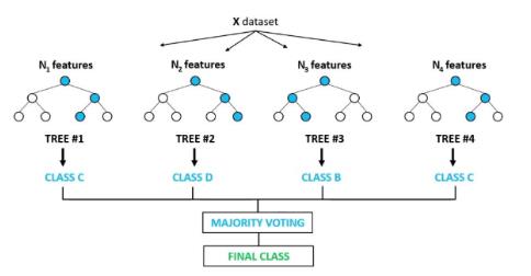
The Random Forest model was employed as a supervised machine learning algorithm for regression, due to its robustness and ability to model non-linear interactions. This ensemble algorithm builds a “forest” of decision trees, where the final prediction is the average of the results from individual trees (Breiman, 2001). The Random Forest architecture is based on Bagging (Bootstrap Aggregating), which creates multiple random training samples with replacement to train each tree, and Random Feature Selection, where a random subset of explanatory variables is considered at each node split of the tree. The process is illustrated in Figure 1.
Figure 1. Diagram of the “Random Forest” model
Source: David (2020)
Hyperparameter optimization (“Grid Search”)
The hyperparameter optimization of the Random Forest model was performed using the Grid Search technique with cross-validation, aiming to maximize predictive capacity and mitigate overfitting (Kuhn and Johnson, 2013). The optimized hyperparameters included: number of estimators (number of trees), maximum depth (tree growth limit), maximum features (number of explanatory variables sampled per node), minimum samples for the node (minimum observations for subdivision), and minimum samples for the leaf (minimum events in a final node).
The best combination of hyperparameters was defined based on the MAE estimator and 3-fold cross-validation, resulting in a maximum depth of 25, maximum features with Square Root, minimum samples for the node of 2, minimum samples for the leaf of 1, and 300 estimators.
Model evaluation
The evaluation of the predictive performance of the models was carried out on the test sample (20% of the data). The statistical metrics used for selecting the best model were the Coefficient of Determination (R²), the Root Mean Squared Error (RMSE), and the Mean Absolute Error (MAE), all reflecting the accuracy on the logarithmic scale of the dependent variable (ln(FRP + 1)).
R² quantifies the proportion of the variability of the dependent variable explained by the model, calculated as:
R² = SSR/SST = 1 – SSRes/SST
where SSR is the Sum of Squares for Regression, SST is the Total Sum of Squares, and SSRes is the Residual Sum of Squares (Montgomery, Peck, and Vining, 2012).
RMSE measures the average magnitude of prediction errors, representing the standard deviation of the residuals, calculated by:
RMSE = sqrt( (1/n) * sum( (yi – y_hat_i)^2 ) )
where n is the number of observations, yi is the actual value and y_hat_i is the predicted value (Hastie, Tibshirani, and Friedman, 2009).
MAE measures the average magnitude of the absolute differences between forecasts and actual values, being calculated by:
MAE = (1/n) * sum( |yi – y_hat_i| )
MAE is less sensitive to outliers than RMSE (Hastie, Tibshirani and Friedman, 2009).
Variable Importance and inference analysis
To understand the determinants of fire intensity, an interpretative analysis of the predictor variables was performed, using specific techniques for each model.
Interpretation in the Econometric Model (Panel)
In the econometric model of Panel Data Regression, the importance of the variables was evaluated by the statistical significance and magnitude of the coefficients, using Student’s t-Test (Wooldridge, 2020). The coefficients were interpreted in terms of elasticity or semi-elasticity, indicating the marginal impact and the direction of the relationship (+/-) with FRP.
Diagnostic tests were applied to validate the statistical inferences. The normality of the residuals was evaluated by the Jarque-Bera test (Jarque and Bera, 1980), and constant variance by the Breusch-Pagan test (Breusch and Pagan, 1979). To correct the diagnosed heteroscedasticity, the final model estimation used Clustered Robust Standard Errors (Wooldridge, 2020).
Interpretation in the “Machine Learning” Model (“Random Forest”)
In the Random Forest algorithm, variable importance was measured by the mean decrease in variance metric, which calculates the total reduction in error provided by each variable across the forest’s trees (Hastie, Tibshirani, and Friedman, 2009). To complement this, SHAP Values analysis (Shapley, 1953; Lundberg and Lee, 2017) was incorporated to quantify the marginal contribution of each variable to individual predictions and identify the directionality of effects (positive or negative).
3. Results and Discussion
Analysis of the Distribution and Treatment of the Target Variable (FRP)
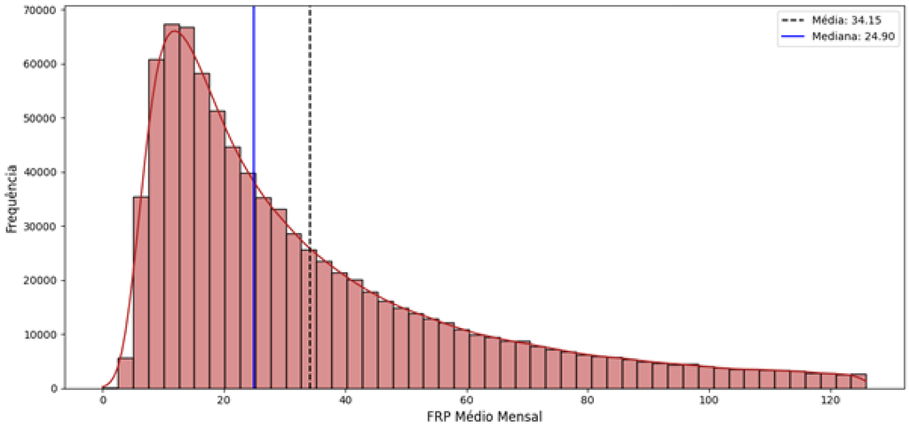
The initial analysis of the Fire Radiative Power (FRP) variable confirmed a high asymmetry in the distribution, with most records concentrating on low energy values. A small number of extreme events, characterized by large-magnitude fires, shifted the mean and increased the variance, as illustrated in Figure 2.
Figure 2. Average Intensity Distribution (FRP)
Source: original research results
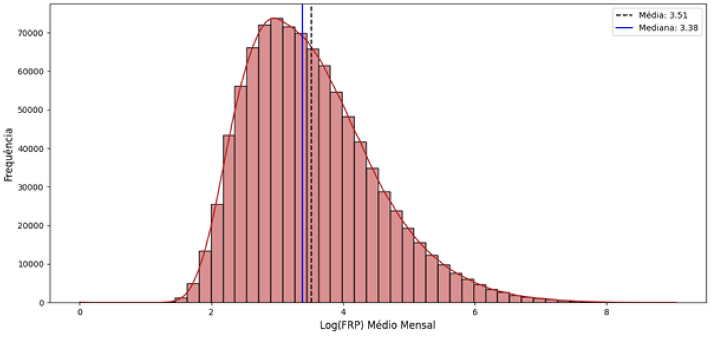
To mitigate this asymmetry and stabilize the variance, the natural logarithmic transformation (ln(FRP + 1)) was applied. This approach proved effective in significantly reducing the range of variation and the disproportionate influence of extreme values, allowing the inclusion of high-magnitude observations in the model without the need for exclusion, as shown in Figure 3.
Figure 3. Average Intensity Distribution (Log FRP)
Source: original research results
Correlations between variables
The Variance Inflation Factor (VIF) test indicated high values for average and maximum temperature, and moderate values for relative humidity, deforestation, and soil moisture. To avoid multicollinearity, the average temperature and soil moisture variables were removed, while maximum temperature and relative humidity were retained to preserve crucial information about temperature peaks and short-term climatic conditions.
Table 1. VIF table for variables
| Variable name | Unit of measure | Type | Description |
|---|---|---|---|
| Latitude | Degree | Decimal value | Latitude where the focus occurred |
| Longitude | Degree | Decimal value | Longitude where the focus occurred |
| Date | Date | Date/Time | Registration date Satellite that performed the focus registration |
| Satellite | Categorical | Text | Name of the Satellite that performed the focus registration |
| State | Categorical | Text | Name of the Brazilian state |
| Municipality | Categorical | Text | Municipality name |
| Biome | Categorical | Text | Biome name |
| Number of days without rain | Days | Integer | Number of days without rain until focus detection |
| Fire risk | Dimensionless | Decimal value | Fire Risk value predicted for the day of the outbreak detection. |
| Radiative power of fire | MW | Decimal value | The power of the detected fire |
Source: original research results
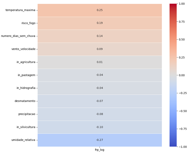
Pearson’s correlation matrix revealed patterns of association between climatic variables and fire intensity. Maximum Temperature (0.25), Fire Risk (0.19), and Number of days without rain (0.14) showed the highest positive correlations with the target variable, suggesting that the energy severity of a fire is directly linked to peak temperature, fire risk, and the dry period. In contrast, relative Humidity (-0.27) demonstrated a negative correlation, indicating it is a factor that contributes to the decrease in fire intensity, according to Figure 4.
Figure 4. Pearson Correlation Matrix
Source: original research results
Temporal dynamics
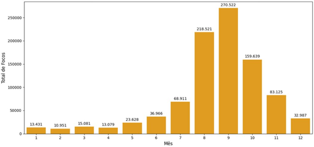
The temporal analysis identified a significant seasonality in the occurrence of fire outbreaks. The lowest levels were observed between January and April, with an increase starting in May, reaching a peak in September and then decreasing. The period from August to October concentrated most of the outbreaks, reinforcing the relevance of the month as a predictive variable for the Random Forest model, as illustrated in Figure 5.
Figure 5. Seasonality: Total Distribution of Hotspots by Month
Source: original research results
Econometric Model of Panel Data
The estimation of the econometric Fixed Effects model, which controlled for unobservable and time-invariant characteristics, explained 18.41% (Rwithin= 0.1841) of the within-panel variability of fire intensity (log FRP) over time. The model coefficients represent percentage growth rates, indicating the percentage increase in FRP for each unit increase in the variable.
The analysis of the coefficients, presented in Table 2, revealed that atmospheric dynamics exert a statistically significant influence (p < 0.01) on fire intensity. Maximum temperature (0.0261) and average wind speed (0.0469) showed positive coefficients, indicating that heat peaks and strong winds increase fire intensity. Relative humidity, in turn, demonstrated a negative relationship (-0.0089) with flame intensity. This dynamic corroborates studies that point to the combination of thermal factors, strong winds, and low humidity as an environment conducive to the intensification of forest fires (Nobre et al., 2016).
The deforestation coefficient (1.3612) was the one with the greatest magnitude and statistical significance (p < 0.01). Em contraste, os coeficientes para as áreas de pastagem, silvicultura e agricultura não apresentaram significância estatística (p > 0.05). This finding suggests that “clearing” fires in areas of recent deforestation consume heavy fuels, releasing larger amounts of energy, while management fires in pastures or agriculture, which consume fine fuels, release radiative energy quickly, without generating structural statistical changes in the order of magnitude of municipal FRP (Roberts et al., 2005). The Student’s t-test confirmed that all variables, with the exception of pasture, silviculture, and agriculture, actually contribute to FRP.
Table 2. Results of the fixed effects model estimation (PanelOLS) for FRP Log
| Variable name | Unit of measure | Type | Description |
|---|---|---|---|
| Year | Year | Integer | Registered year |
| Municipality ID | Categorical | Integer | Municipality identifier code |
| Biome | Categorical | Text | Biome name |
| Total area | Km² | Decimal value | Total area of the biome in the municipality |
| Deforested | Km² | Decimal value | Deforested area of the biome in the municipality |
| Hydrography | Km² | Decimal value | Hydrography area of the biome in the municipality |
Source: original research results
Random Forest Model
The Random Forest model was developed using the FRP log as the dependent variable and a set of features that included maximum temperature, relative humidity, wind speed, precipitation, number of rainless days, fire risk, deforestation, pasture indices, silviculture, agriculture, hydrography, and month. Hyperparameter optimization was performed via Grid Search with cross-validation, according to the options presented in Table 3.
Table 3. Hyperparameter grid used in “Grid Search”
| Variable name | Unit of measure | Type | Description |
|---|---|---|---|
| Municipality ID | Categorical | Integer | Municipality identifier code |
| Name | Categorical | Text | Municipality name |
| State | Categorical | Text | Name of the Brazilian state |
Source: original research results
The best performing model, after optimization, resulted in an R² explanatory power of 0.3626, with a Mean Absolute Error (MAE) of 0.62 and a Root Mean Squared Error (RMSE) of 0.79 on the test set. The error reflects logarithmic units. When returning to the original scale, the MAE indicates that the model’s predictions deviate, on average, by a factor of approximately 1.8, being able to anticipate the order of magnitude of the fire. The proximity between RMSE and MAE values suggests the absence of extreme and systemic outliers in the predictions, indicating predictive consistency around the mean error (Chai and Draxler, 2014). Although the R² is relatively low, capturing more than a third of the variance in complex and uncontrolled ecological systems may indicate that the model has mapped structural drivers (Moller and Jennions, 2002).
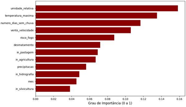
The main variables that impact fire intensity, according to the importance level of the Random Forest model, were relative humidity, maximum temperature, and number of days without rain, as shown in Figure 6.
Figure 6. Variables with the greatest impact on fire intensity
Source: original research results
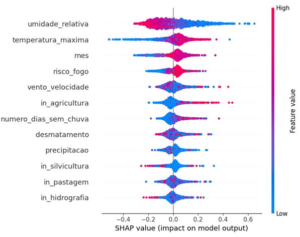
The analysis of SHAP Values complemented the understanding of the directionality of these impacts. Relative humidity proved to be a strong factor in decreasing fire intensity, while maximum temperature and the number of days without rain contributed positively to increasing intensity, as shown in Figure 7. Values closer to red indicate a high value in the variable and a positive impact on FRP, while blue values indicate a low value in the variable and a negative impact.
Figure 7. SHAP values of the model variables
Source: original research results
The identification of these main drivers of high-intensity fires enables the planning of preventive strategies and the early allocation of contingency resources. The developed modeling allows for predicting the order of magnitude of events, contributing to a more agile and effective mobilization in combating large-scale fires.
In summary, the results of both models indicated the influence of drought, wind, and temperature conditions on fire intensity, in addition to the significant impact of deforestation. These findings demonstrate that high-severity fires result from the overlap of macroclimatic extremes and the availability of fuel from recent deforestation. With access to information and predictive models, it is possible to act in the prevention and control of these phenomena.
4. Conclusion
This study aimed to develop a machine learning model to estimate the Fire Radiative Power (FRP) of fire hotspots in Brazil, using data from the National Institute for Space Research (INPE) and complementary environmental variables, identifying the most important factors for its determination. It was found, through a panel data econometric model, that the deforestation index exerted the greatest positive and structural impact on fire intensity, while areas of agriculture, pasture, and forestry showed no statistical significance. Complementarily, predictive modeling with the Random Forest algorithm demonstrated that climatic conditions have a significant impact on fire propagation and intensity. Relative air humidity was identified as the main mitigating factor, while maximum temperature and the number of rainless days acted as the greatest catalysts. The results of both models converged in indicating that high-severity fires result from the overlap of macroclimatic extremes combined with fuel availability from recent deforestation.
The main contribution of this work lies in offering a quantitative decision support tool for environmental management and civil defense agencies, enabling the prediction of the order of magnitude of fire events and, consequently, a more agile and effective mobilization in combating large-scale outbreaks. The identification of the main vectors of high-intensity fires facilitates the planning of preventive strategies and the early allocation of contingency resources. However, a limitation of the study stemmed from resource availability, which prevented the amplification of the number of variables and the increase in the years considered for the analysis. For future studies, it is suggested to explore a more comprehensive set of variables and an extended historical series, which could further refine the predictive and explanatory capacity of the models.
Bibliographic References
Breiman, L. 2001. Random Forests. Machine Learning 45(1): 5-32.
CNN Brasil. 2025. Brasil registrou 278,3 mil focos de incêndio em 2024, diz Inpe. Disponível em: https://www.cnnbrasil.com.br/nacional/brasil-registrou-2783-mil-focos-de-incendio-em-2024-diz-inpe/. Acesso em: 28 set. 2025.
David, Davis. Random forest classifier tutorial: how to use tree-based algorithms for machine learning. freeCodeCamp, 6 ago. 2020. Disponível em: https://www.freecodecamp.org/news/how-to-use-the-tree-based-algorithm-for-machine-learning/. Acesso em: 14 abr. 2026.
Guimarães, P. P.; Souza, S. M.; Fiedler, N. C.; Silva, A. G. 2014. Análise dos Impactos Ambientais de um Incêndio Florestal. Agrarian Academy 1(1): 38-60.
Hair Jr., J. F.; Black, W. C.; Babin, B. J.; Anderson, R. E.; Tatham, R. L. 2009. Análise Multivariada de Dados. 6. ed. Bookman, Porto Alegre, RS, Brasil.
Hausman, Jerry A. Specification tests in econometrics. Econometrica, v. 46, n. 6, p. 1251-1271, 1978.
INPE (Instituto Nacional de Pesquisas Espaciais). Programa Queimadas: Monitoramento dos Focos Ativos por Satélite. Disponível em: http://terrabrasilis.dpi.inpe.br/queimadas/portal/pages/secao_informacoes/faq/. Acesso em: 26 jan. 2026.
Juvanhol, R. S.; Fiedler, N. C.; Santos, A. R.; Peluzio T. M. O.; Silva W. B.; Pinheiro C. J. G; Sousa H. C. P. 2023. Use of machine learning as a tool for determining fire management units in the brazilian atlantic forest. Anais da Academia Brasileira de Ciências 95(2): e20201039.
Kuhn, M.; Johnson, K. Applied Predictive Modeling. Nova York: Springer, 2013.
Montgomery, D. C.; Peck, E. A.; Vining, G. G. 2012. Introduction to Linear Regression Analysis. 5. ed. Wiley, Hoboken, NJ, USA.
Nobre, C. A.; Sampaio, G.; Borma, L. S.; Castilla-Rubio, J. C.; Silva, J. S.; Cardoso, M. 2016. Land-use and climate change risks in the Amazon and the need of a novel sustainable development paradigm. Proceedings of the National Academy of Sciences 113(39): 10759-10768.
Roberts, G.; Wooster, M. J.; Perry, G. L. W.; Kaufman Y. J. 2005. Retrieval of biomass combustion rates and totals from fire radiative power observations: FRP derivation and calibration relationships between biomass consumption and fire radiative energy release. Journal of Geophysical Research: Atmospheres 110(D24311).
Shumway, R. H.; Stoffer, D. S. Time Series Analysis and Its Applications: With R Examples. 4. ed. Cham: Springer, 2017
Viganó, H. H. G.; Souza, C. C.; Cristaldo, M. F.; Jesus, L. 2017. Redes Neurais Artificiais na Previsão de Queimadas e Incêndios no Pantanal. Revista Brasileira de Geografia Física 10(5): 1355-1367.
Wooldridge, J. M. Econometric Analysis of Cross Section and Panel Data. 2. ed. Cambridge: MIT Press, 2010.
Wooster, M. J.; Roberts, G.; Perry, G. L.; Drake, N.; Rebelo, L. M.; Dipotso, F. 2005. Retrieval of fire radiative energy from MODIS: Application to southern African savanna fires using geostationary SEVIRI imagery. Journal of Geophysical Research: Atmospheres 110(D21111).
Article originating from the Course Conclusion Work of the Specialization in Data Science and Analytics of the MBA USP/Esalq
To learn more about the course, click here and access the MBX Academy platform