
September 10, 2026
Hedonic Pricing of Real Estate in Greater Florianópolis: Use and Comparison of “Machine Learning” Models
Gabriel Galvan de Cesaro; Lilian Cristina Da Silveira
DOI: 10.22167/2675-6528-202602220
Article derived from a Final Course Work (TCC), with content based on the student’s original work and adapted to the editorial format of the Revista E&S with the support of the ResumeAI tool, an artificial intelligence solution developed by the Pecege Institute for textual synthesis and organization.
Summary
The real estate market in Greater Florianópolis has experienced accelerated appreciation, driven by population growth and tourism and investment demand. This study analyzed the determinants of residential property values and compared the predictive performance of machine learning models, specifically Random Forest and Gradient Boosting (XGBoost), with Ordinary Least Squares (OLS) regression. Data were collected via web scraping from two real estate portals in March 2026, covering the municipalities of Florianópolis, São José, Palhoça, and Biguaçu, resulting in 8,056 valid observations after cleaning. Model performance was evaluated using R², RMSE, and MAPE metrics. XGBoost showed the best overall predictive performance (R² = 0.742, RMSE = R$ 927,113), while Random Forest achieved the lowest relative error (MAPE = 25.69%). The main price determinants identified were built area, location region, and number of bathrooms. A complementary analysis by market segment revealed that OLS depended on extreme values to sustain its fit, while ensemble models maintained stable performance. It was concluded that machine learning methods are more robust for hedonic pricing in heterogeneous real estate markets, especially in the presence of atypical properties.
Keywords: Ensemble; Real Estate; Regression; Residential; Web Scraping.
1. Introduction
The real estate market in Greater Florianópolis has experienced accelerated appreciation, driven by population growth and the pressure of tourist and investment demand. Florianópolis, despite being the 21st capital in absolute population, registered the third largest relative growth between 2010 and 2022, with a 27.5% increase in its population (IBGE, 2022). This dynamic is reflected in property prices, which had an accelerated increase of about nine percent between January and December 2024 (FIPE, 2024).
The neighboring cities, such as São José, Palhoça, and Biguaçu, also showed relative population growth in the same proportion as the capital (IBGE, 2022). However, their prices per square meter are lower; São José, for example, ended 2024 with a value 32% below the average for Florianópolis (FIPE, 2024), offering more affordable housing alternatives for workers from the Santa Catarina island. In this scenario, purchasing a property is often the largest financial transaction for most people (Pedersen et al., 2013), making it crucial to understand market pricing mechanisms.
Knowing how the market prices similar assets allows the buyer to identify opportunities and avoid overvalued properties. For the seller, an accurate estimate of market value can optimize return on investment and speed up the sale, avoiding under- or overvaluation of the asset (Moro, 2017). One of the established methods for estimating property prices is hedonic pricing, which, according to Fávero (2003), uses regression models to define prices based on the characteristics of residences.
The hedonic term derives from hedonism, indicating that consumer pleasure or satisfaction depend on the attributes of the acquired good (Fávero et al., 2008). Rosen (1974) describes hedonic prices as implicit prices of attributes, determined by the characteristics and prices associated with different products. Thus, hedonic pricing postulates that the final price is the sum of the prices of the attributes, evidencing the individual contribution of each characteristic of the property.
Given the complexity and rapid appreciation of the real estate market in Greater Florianópolis, it becomes relevant to improve pricing tools. This study seeks to contribute to the advancement of academic literature by estimating the value of residential properties in the Greater Florianópolis region (comprising the municipalities of Florianópolis, São José, Palhoça, and Biguaçu) based on data collected via web scraping from online real estate advertisement platforms. To this end, the performance of an ordinary least squares method (OLS) regression, used as a reference model, is compared with that of machine learning algorithms, specifically Random Forest (Breiman, 2001) and Gradient Boosting through XGBoost (Chen and Guestrin, 2016).
2. Material and Methods
All data collection, processing, and modeling steps were implemented in Python 3.12, executed in a Windows 11 environment. The libraries used included “Requests” and “BeautifulSoup” for data collection, “Pandas” for manipulation, “Statsmodels” and “Scikit-learn” for hedonic regression and “random forest”, “XGBoost” for “gradient boosting” and SHAP for model interpretation.
The data were obtained through “web scraping” from two local real estate portals in the Greater Florianópolis region (Florianópolis, São José, Palhoça, and Biguaçu) in March 2026, exclusively covering residential properties advertised for sale. The choice for online listing data was due to the unavailability of official sales records, and the option for local real estate agencies was made due to the privacy policies of multi-real estate portals that prohibit automated collection.
Data collection for Imobiliária A’s portal used an internal REST API that returned data in JSON format, consumed directly by a Python “scraper” with the Requests library. For Imobiliária B’s portal, which did not have a public API, the process was divided into two stages: requesting listing pages with “Requests” and “BeautifulSoup” for basic attributes, and visiting each individual property page with a “Chromium” browser controlled by the “Playwright” library for extracting complementary variables loaded dynamically via JavaScript. Finally, the databases were consolidated into a single CSV file, totaling 8,156 records before cleaning.
The consolidated raw data were subjected to a cleaning process to remove records with registration errors, unrealistic values, or insufficient information. Initially, 15 types of properties were standardized into two subdivisions: “apartment” or “house”. Properties without a parking space were treated as 0. Records with missing number of bedrooms or bathrooms, sale price below R$ 90,000, built area less than 10m², more than 9 bedrooms, more than 12 parking spaces, or size above 1000 m² were disregarded.
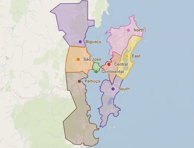
The neighborhood and city fields underwent normalization, and a new “region” field was created. For Florianópolis, the neighborhoods were classified into Central, Continental, East, North, and South regions, according to Complementary Law No. 739 (FLORIANÓPOLIS, 2023). For the other municipalities (Biguaçu, Palhoça, and São José), the “region” field was filled with the city’s name itself, as shown in the simplified representation in Figure 1.
Figure 1. Regions considered for the study
Source: Own elaboration, based on Google Maps
The amenities collected in free text format were converted into seven binary variables: pool, balcony, barbecue grill, furnished property, elevator, gym, and party room, by searching for predefined terms. After all cleaning steps, the final dataset had 8,056 valid observations and the variables presented in Table 1.
Table 1. Database variables
| Name | Description | Type |
|---|---|---|
| real estate agency | Real estate agency name | Classification |
| type | Property type | Classification |
| street | Street name | Nominal |
| neighborhood | Property neighborhood | Nominal |
| city | Property city | Classification |
| size_m2 | Size in m² | Continuous quantitative |
| rooms | Number of bedrooms | Discrete quantitative |
| bathrooms | Number of bathrooms | Discrete quantitative |
| vacancies | Number of garage parking spaces | Discrete quantitative |
| value | Property price in R$ | Continuous quantitative |
| region | Property region | Classification |
| swimming pool | Presence of swimming pool | Binary/Logic |
| balcony | Presence of balcony/veranda | Binary/Logic |
| barbecue grill | Presence of barbecue grill | Binary/Logic |
| furnished property | Furnished property | Binary/Logic |
| elevator | Elevator presence | Binary/Logic |
| academic world | Presence of academia | Binary/Logic |
| party room | Presence of party room | Binary/Logic |
Source: Original research results
The first estimated model was a linear regression by Ordinary Least Squares (OLS), used as a reference model. The dependent variable, “value” (property price in reais), was transformed to the logarithmic scale, a procedure equivalent to the Box-Cox transformation with parameter λ=0, seeking distribution normalization. The final model specification was validated by the “stepwise” procedure with an elimination criterion when p-value > 0.05, removing the “imovel_mobiliado” variable.
The machine learning models adopted were “Random Forest” (Breiman, 2001) and “Gradient Boosting” through the “XGBoost” implementation (Chen and Guestrin, 2016). For the machine learning models, the database was divided into a training set (80% of observations, n = 6,444) and a test set (20% of observations, n = 1,612). Hyperparameter selection was performed by RandomizedSearchCV, using k-fold cross-validation with k = 5 on the training set and RMSE as the optimization criterion. 40 hyperparameter combinations were sampled, presented in Table 2.
Table 2. Hyperparameters selected by RandomizedSearchCV
| Hyperparameter | Description | Random Forest | XGBoost |
|---|---|---|---|
| n_estimators | Number of trees | 300 | 200 |
| maximum depth | Maximum depth of each tree | 30 | 6 |
| max_features | Fraction of variables evaluated in each split | 0,5 | |
| min_samples_split | Minimum number of samples to split a node | 5 | |
| min_samples_leaf | Minimum number of samples in each leaf | 2 | |
| rate of learning | Learning rate (weight of each tree) | 0,05 | |
| secondary sample | Fraction of observations used by trees | 0,6 | |
| colsample_bytree | Fraction of variables used by tree | 0,8 | |
| gamma | Minimum gain to perform a split | 0,1 | |
| min_child_weight | Minimum weight in each node | 1 |
Source: Original research results
The three models were evaluated on the test set by the metrics R², RMSE, MAE, and MAPE, all calculated on the original scale in reais, reversing the logarithmic transformation with the exponential function before calculation.
The analysis of the Variance Inflation Factors (VIF) of the initial OLS specification revealed severe multicollinearity between `log_size_m2` (VIF = 63.97) and `rooms` (VIF = 17.60), recognized as a limitation of Model A, selected after testing three specifications to address this issue. The OLS model was estimated with robust HC3 standard errors. Heteroscedasticity was detected by the Breusch-Pagan test and corrected by applying robust HC3 standard errors as a methodological precaution.
3. Results and Discussion
Exploratory Analysis
After the collection and sanitization steps, the final database contained 8,056 observations of residential properties advertised for sale in the Greater Florianópolis region. The descriptive statistics of the study’s numerical variables are presented in Table 3.
Table 3. Descriptive statistics of the numerical variables
| Variable | average | median | standard deviation | min | max |
|---|---|---|---|---|---|
| size_m2 (m²) | 143,05 | 106,0 | 111,3 | 11,0 | 1000,0 |
| rooms | 2,73 | 3 | 1,09 | 1 | 9 |
| bathrooms | 2,54 | 2 | 1,37 | 1 | 12 |
| vacancies | 1,68 | 1 | 1,19 | 0,0 | 12 |
| value (R$) | 1.655.513 | 1.100.000 | 1.959.595 | 90.000 | 50.000.000 |
| _price_m2 (R$/m²) | 11.895 | 10.328 | 7095 | 490,2 | 138.183,3 |
Source: Original research results
The high standard deviation observed for size_m2 (111.3 m²) and value (R$ 1,959,595) reflects the heterogeneity of the database, which brings together property types and regions with very distinct characteristics. For exploratory purposes, the price per square meter (R$/m²) was used to compare the value of properties of different sizes under more homogeneous conditions, revealing differences in appreciation between regions and types that the analysis of absolute value could mask. This variable is used exclusively in the exploratory analysis, while the modeling adopts log(value) as the dependent variable and log(size_m2) as one of the predictor variables.
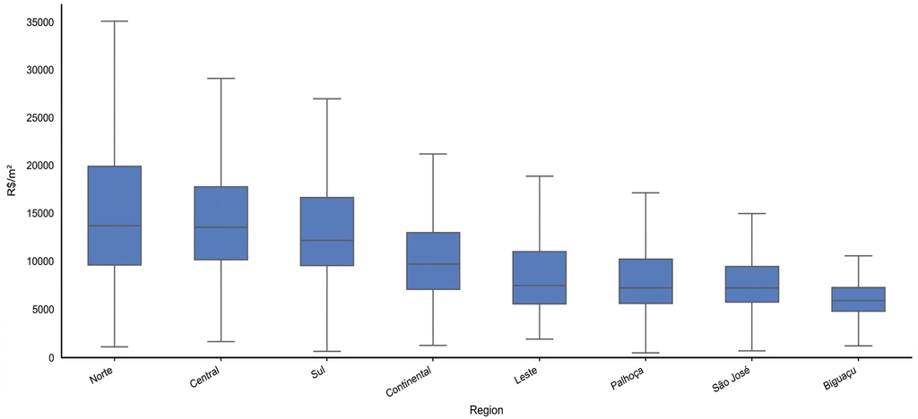
The median price per square meter by region, as shown in Figure 2, reveals significant differences within the municipality of Florianópolis. The North and South regions present the highest median values, followed by the Central region, while the municipalities of Greater Florianópolis (São José, Palhoça, and Biguaçu) systematically show lower prices per square meter. The difference between the most valued and least valued region is approximately 130%. This gradient is consistent with FipeZap index data and reflects the pattern documented in the literature that proximity to the coast and places of interest are relevant determinants of the hedonic value of real estate in coastal cities (Dantas et al., 2007). This result also anticipates the regional premiums estimated by the hedonic model.
Figure 2. Price per m² by region with extreme outliers hidden
Source: Original survey data
The neighborhood analysis within the North region reveals that the dispersion of the price per square meter persists even in the most valued region. Jurerê presents a median cost of R$ 24,000/m², while Vargem Grande registers R$ 8,000/m², a difference of 200%. This indicates that the region variable captures part of the price heterogeneity, but not all of it, as high-standard neighborhoods concentrate appreciation attributes not entirely observable in the listings, such as finishing quality and construction standard.
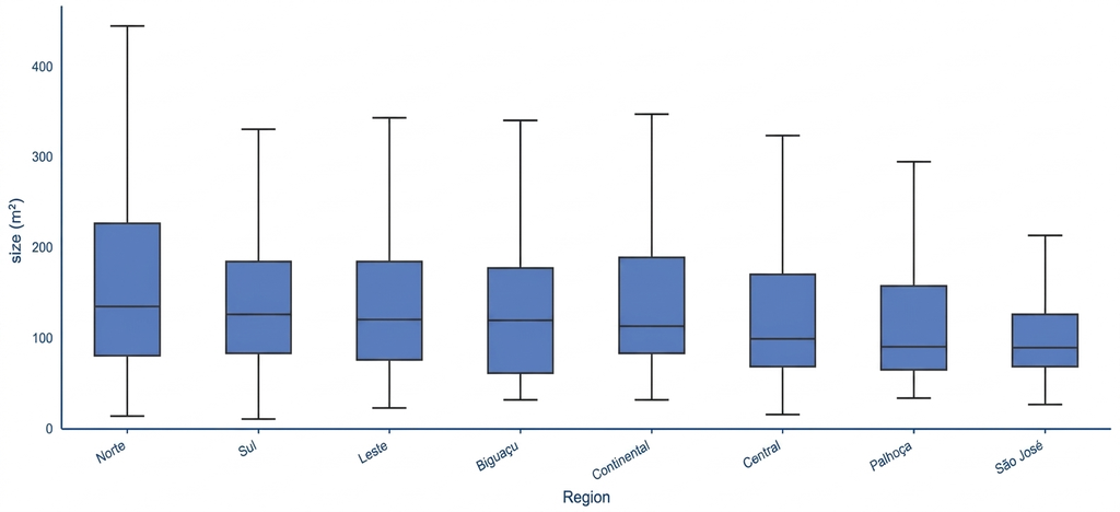
The comparison of property sizes by region, presented in Figure 3, reveals that the North region also leads in median size and shows the largest standard deviation. This dispersion is explained by the coexistence, within the same region, of high-standard neighborhoods (such as Jurerê and Jurerê Internacional, with large properties) and neighborhoods with a more popular profile (such as Vargem Grande), where properties are significantly smaller.
Figure 3. Size in m² by region with extreme outliers hidden
Source: Original survey data
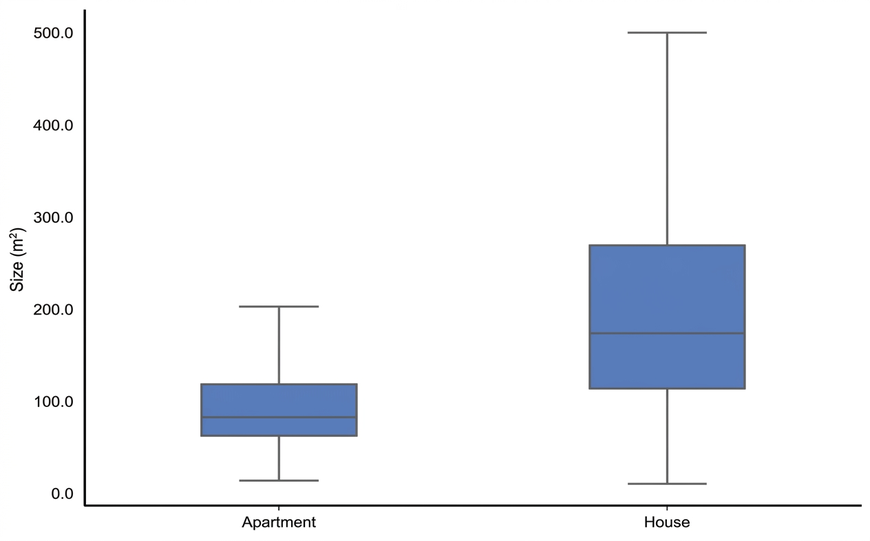
Figure 4 breaks down this variation by property type and shows that houses have a considerably larger median size than apartments, with equally higher dispersion. This result suggests that part of the standard deviation observed in the size_m2 variable stems from the heterogeneous composition of the sample between the two types, reinforcing the need to simultaneously control for type and region in the estimated models, which is done through dummy variables included in the hedonic specification.
Figure 4. Size in m² by property type with extreme outliers hidden
Source: Original survey data
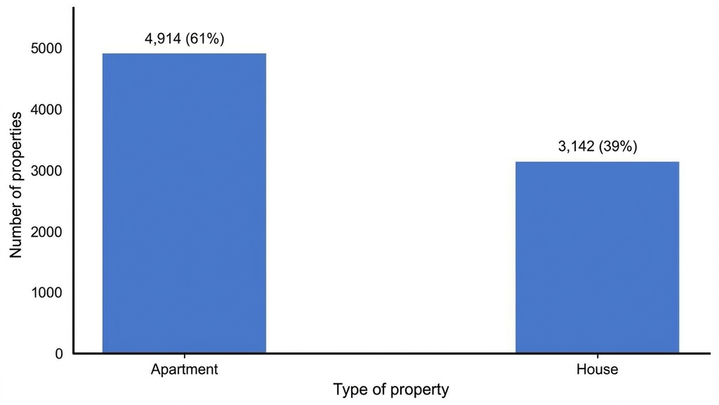
The distribution by property type revealed a predominance of apartments (61%) over houses (39%), according to Figure 5. This discrepancy compared to the IBGE survey (IBGE, 2022) for Florianópolis (56.01% houses and 43.99% apartments) is expected, as the database captures properties actively advertised for sale on digital portals, where apartments have greater representation, reflecting market flow rather than the total stock of households.
Figure 5. Count by property type
Source: Original survey data
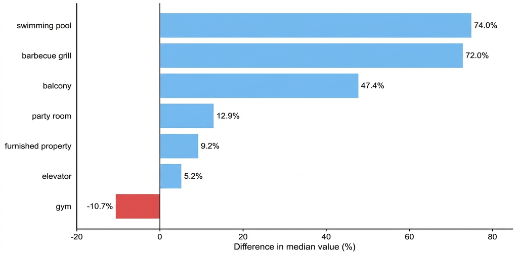
Among the collected amenities, barbecue grill is the most prevalent in the sample (69.8%), followed by party room (39.9%) and swimming pool (39.7%). Figure 6 shows the percentage difference between the median value of properties that have each amenity and the median value of those that do not, without controlling for other variables.
Figure 6. Difference in median value between properties with and without amenities
Source: Original survey data
Pool (+74.0%) and barbecue area (+72.0%) show the largest positive impacts on the median value, followed by balcony (+47.4%), while gym shows a negative result (-10.7%). The latter does not indicate a devaluation effect, but reflects a confounding effect, as gyms are more present in mid-range condominiums, which may be located in less valued regions. This limitation of the raw analysis is corrected by the regression model, which estimates the effect of each attribute while simultaneously controlling for the other variables.
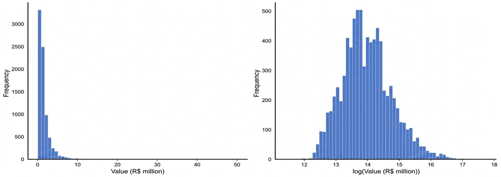
OLS regression assumes that the model’s residuals follow an approximately normal distribution. In real estate data, property values typically do not follow a normal distribution pattern, exhibiting pronounced positive skewness due to the presence of a few very high-end properties. The logarithmic transformation is a common approach in hedonic literature to address this issue (Rosen, 1974; Malpezzi, 2003), compressing the right tail, reducing skewness, and stabilizing the variance of the residuals.
Figure 7 presents the distribution of the property value before and after the logarithmic transformation. The original value showed a skewness of 6.58, characterizing a distribution with a long right tail. After the transformation, the skewness reduced to 0.46, substantially approximating the distribution to symmetry.
Figure 7. Distribution of the property value before and after logarithmic transformation
Source: Original survey data
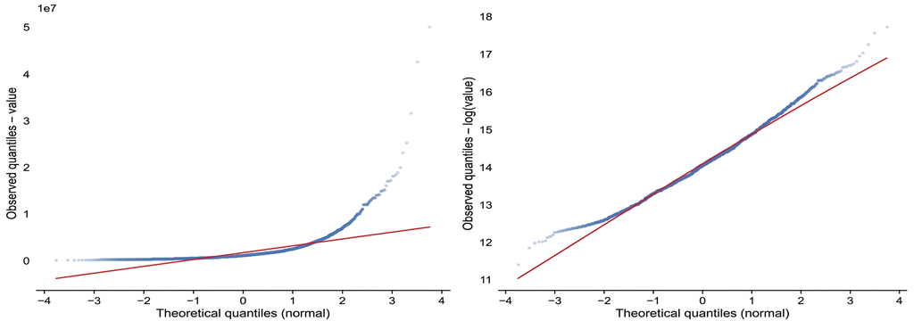
Normality was assessed by the Shapiro-Francia test, which rejected normality for both the original and log(value) values, an expected result in large samples (Field, 2018). The QQ-plots (theoretical versus observed quantiles graphs) in Figure 8 show that the logarithmic transformation markedly reduced the asymmetry of the dependent variable, bringing its distribution closer to normality. This condition favors the fulfillment of the normality assumption for the residuals, formally verified in the OLS model diagnostics section.
Figure 8. QQ-plots of the dependent variable before and after logarithmic transformation
Source: Original survey data
The tamanho_m2 predictor showed an asymmetry of 2.35, also high, and was also transformed to log(tamanho_m2). The categorical variables region and type were encoded as dummy variables, with Biguaçu and Apartment as reference categories, respectively.
Spearman’s correlation analysis between the numerical variables and the property value indicated that size_m2 presents the highest correlation (p = 0.733, p < 0.001), followed by bathrooms (p = 0.690), bedrooms (p = 0.580), and parking spaces (p = 0.556). This ordering is consistent with the analysis by Sirmans et al. (2005), which identified built area and number of bathrooms as the most frequently significant and largest attributes in residential hedonic models.
Ordinary Least Squares Regression
The analysis of the Variance Inflation Factors (VIF) of the initial specification revealed severe multicollinearity between log_size_m2 (VIF = 63.97) and rooms (VIF = 17.60), indicating that the two variables capture overlapping dimensions of the property. Multicollinearity does not bias coefficients but inflates their standard errors, reducing the power of hypothesis tests (Fávero and Belfiore, 2024). To evaluate alternatives, three specifications were tested to address multicollinearity. Model A (original specification, with log_size_m2 and rooms separated) was selected for presenting the lowest AIC (7.337) and the highest adjusted R² (0.7636) among the three specifications, as shown in Table 4. Models B (without rooms) and C (replacing size and rooms with m²/room) presented higher AICs and slightly lower adjusted R², and were discarded. The multicollinearity between log_size_m2 and rooms is recognized as a limitation of Model A and is reported by the VIF analysis.
Table 4. VIF analysis result
| Model | number of predictors | Adjusted R² | PCA | Maximum VIF |
|---|---|---|---|---|
| The (original) | 19 | 0,7636 | 7337 | 63,97 |
| B (no rooms) | 18 | 0,7635 | 7358 | 51,30 |
| C (m²/room) | 18 | 0,7143 | 8881 | 41,51 |
Source: Original research results
The OLS model estimated with HC3 robust standard errors presented an R² of 0.764, indicating that the included variables explain 76.4% of the variation in the logarithm of real estate prices. This result falls within the typical range reported in the literature (Sirmans et al., 2005). The F-statistic rejected the null hypothesis that all coefficients are jointly equal to zero (F = 1.168, p < 0.001), confirming the overall significance of the model. Table 5 presents the estimated coefficients.
Table 5. OLS model coefficients
| Variable | Coefficient (β) | Standard Deviation | p-value |
|---|---|---|---|
| Intercept | 9,7961 | 0,0510 | 0,0000 |
| central region | 0,6431 | 0,0291 | 0,0000 |
| continental_region | 0,3921 | 0,0308 | 0,0000 |
| east region | 0,3571 | 0,0308 | 0,0000 |
| north_region | 0,7475 | 0,0296 | 0,0000 |
| palhoca_region | 0,2228 | 0,0299 | 0,0000 |
| south_region | 0,7189 | 0,0301 | 0,0000 |
| sao_jose_region | 0,1994 | 0,0295 | 0,0000 |
| house_type | -0,1905 | 0,0141 | 0,0000 |
| log_size_m2 | 0,6803 | 0,0119 | 0,0000 |
| rooms | -0,0296 | 0,0062 | 0,0000 |
| bathrooms | 0,1303 | 0,0048 | 0,0000 |
| vacancies | 0,0625 | 0,0045 | 0,0000 |
| swimming pool | 0,1826 | 0,0097 | 0,0000 |
| balcony | 0,0489 | 0,0099 | 0,0000 |
| barbecue grill | 0,0291 | 0,0103 | 0,0046 |
| elevator | 0,1234 | 0,0127 | 0,0000 |
| academic world | 0,0299 | 0,0144 | 0,0373 |
| party room | 0,0435 | 0,0117 | 0,0207 |
Source: Original research results
The imovel_mobiliado variable was removed by the stepwise procedure (p = 0.054) and does not integrate the final model. The other coefficients remained unchanged.
Regional variables, with Biguaçu as the reference category, reveal significant location premiums. Converting the coefficients to exact percentage variation, properties in the North region of Florianópolis are worth about 111% more than equivalent properties in Biguaçu, followed by the South (+105%) and Central (+90%) regions. The magnitude of these regional premiums, which can exceed 100%, is significant and suggests that the location variable is the main determinant of real estate value in Greater Florianópolis, overriding the physical characteristics of the property.
Among the physical variables of the property, the number of bathrooms shows the highest positive coefficient (β = 0.130), implying an increase of approximately 13.9% in value for each additional bathroom, controlling for other variables. This is a result consistent with the range of 10% to 12% documented by Sirmans et al. (2005) for North American markets. Parking spaces contribute an additional 6.4% per unit (β = 0.063). The house_type coefficient (β = -0.190) indicates that houses are worth approximately 17.4% less than apartments of equivalent size, region, and amenities, reflecting the higher relative valuation of apartments in the online advertised market, concentrated in dense urban areas where this type predominates. Among amenities, a swimming pool registers the highest implicit premium (+20.0%), followed by an elevator (+13.1%), a party room (+4.4%), a gym (+3.0%), and a barbecue grill (+2.9%), a result consistent with the review by Sirmans et al. (2005), which identified swimming pools and garages as the amenities with the highest frequency of positive and significant coefficients in residential hedonic studies.
The negative coefficient for bedrooms (-0.030), controlling for size, finds a parallel in the literature: Sirmans, Macpherson, and Zietz (2005) observed that the sign for bedrooms tends to become negative or non-significant when the built area is included simultaneously in the model, as the two variables capture overlapping dimensions of the property. This result is interpreted as a penalty for small bedrooms: starting from a fixed size of a property, a larger number of bedrooms implies a smaller average area per room. Table 6 presents the VIFs of the model, confirming severe multicollinearity between log_size_m2 (VIF = 63.97) and bedrooms (VIF = 17.60), recognized as a limitation.
Table 6. Variance Inflation Factors (VIF) of the selected model
| Variable | VIF |
|---|---|
| log_size_m2 | 63,97 |
| rooms | 17,60 |
| bathrooms | 10,32 |
| vacancies | 4,67 |
| barbecue grill | 4,02 |
| house_type | 3,98 |
| central region | 3,71 |
| elevator | 3,46 |
| party room | 2,98 |
| north_region | 2,65 |
| sao_jose_region | 2,29 |
| swimming pool | 2,10 |
| south_region | 2,09 |
| continental_region | 2,03 |
| palhoca_region | 2,01 |
| balcony | 1,92 |
| east region | 1,83 |
| academic world | 1,28 |
Source: Original research results
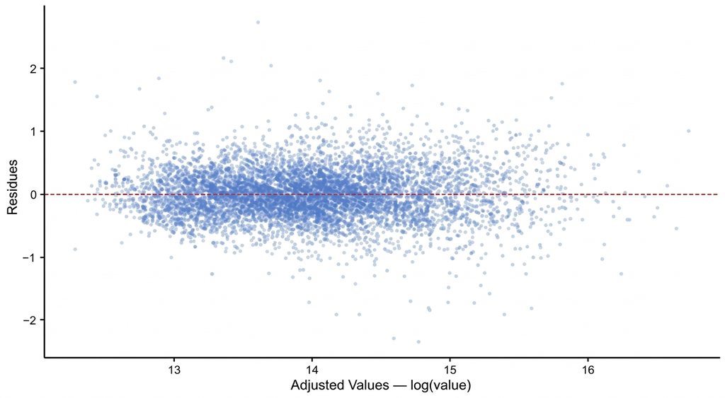
The heteroscedasticity detected by the Breusch-Pagan test (LM = 490.15, p < 0.001) is expected in hedonic models, documented in relation to both the age and the value of the properties (Goodman and Thibodeau, 1995; Malpezzi, 2003). The correction by robust standard errors HC3 does not alter the estimated coefficients, only the standard errors and confidence intervals, preserving the validity of the inference. The plot of residuals versus fitted values, presented in Figure 9, does not show a visual pattern of pronounced heteroscedasticity, which is common in large samples where the Breusch-Pagan test detects statistically significant but practically small deviations. The correction by robust standard errors HC3 was applied as a methodological precaution, preserving the validity of the inference.
Figure 9. Residuals versus Fitted Values
Source: Original survey data
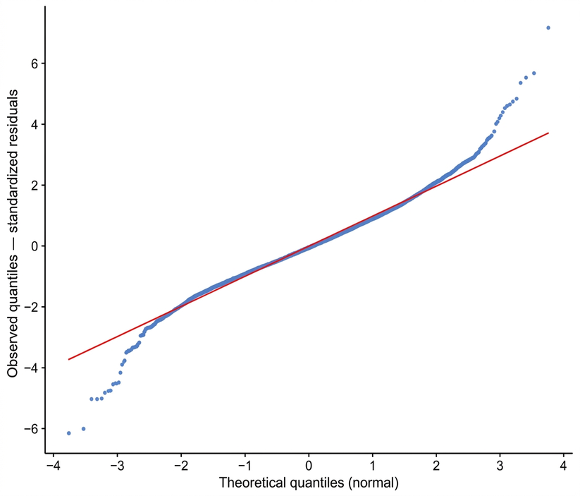
The excess kurtosis of the residuals (2.28) indicates heavier tails than the normal distribution, suggesting less precise performance at the extremes of the price distribution. This result is verified in the QQ-plot of the standardized residuals in Figure 10, where the points at the ends deviate from the reference line, and motivated the complementary analysis by market segment presented in the following section.
Figure 10. QQ-Plot (Quantile-Quantile Plot) of standardized residuals
Source: Original survey data
Machine Learning Models
Table 7 presents the performance metrics of the three models on the test set, calculated on the original scale in reais after reversing the logarithmic transformation. For purposes of equivalent comparison with the machine learning models, the ordinary least squares method was re-evaluated on the same 20% test set of observations, obtaining R² = 0.717. The value, lower than the R² of 0.764 presented in the previous section, is an expected difference, given that the latter was calculated on all 8,056 observations used for fitting, while this refers to data that the model had not seen during training.
Table 7. Comparison of metrics between models for the test set
| Model | R² Test | RMSE (BRL) | MAPE |
|---|---|---|---|
| OLS | 0,7168 | 971.153 | 29,17% |
| Random Forest | 0,7339 | 941.302 | 25,69% |
| XGBoost | 0,7419 | 927.113 | 26,27% |
Source: Original research results
The ensemble models outperformed the ordinary least squares method in all evaluated metrics. XGBoost showed the best performance in R² (0.742) and RMSE (R$ 927,113), while Random Forest achieved the lowest MAPE (25.69%), indicating a lower relative error in intermediate-value properties. The RMSE of R$ 927,113 represents approximately 84% of the median property value in the sample (R$ 1,100,000), reflecting the structural heterogeneity of the market discussed in the exploratory analysis, rather than a model failure.
The observed pattern, with XGBoost slightly superior in global metrics and Random Forest more precise in relative error, reflects the structural differences between the two algorithms: XGBoost, by building trees sequentially with a focus on reducing accumulated residual, tends to minimize global quadratic error, while Random Forest, by aggregating independent trees trained on distinct samples, presents lower variance in individual predictions (Breiman, 2001; Chen and Guestrin, 2016). The residual MAPE of 25% to 29% is consistent with that reported in Brazilian hedonic studies with listing data (Kappel and Teodoro, 2021). The variance not explained by the models is inherent to the nature of the data, as characteristics determining individual value, such as state of conservation, quality of finish, solar orientation, and floor, are not systematically reported in listings and therefore cannot be included in the models (Malpezzi, 2003; Campos, 2017).
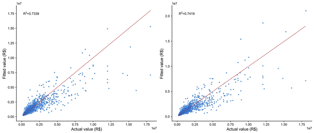
Figure 11 presents the actual versus predicted values for Random Forest and XGBoost on the test set. In both models, the points concentrate near the diagonal for intermediate-value properties, with greater dispersion at the extremes of the distribution, a pattern consistent with the high MAPE and the kurtosis of the residuals observed in OLS, which motivated the complementary analysis by market segment presented in the following section.
Figure 11. Actual versus predicted values for Random Forest and XGBoost on the test set
Source: Original survey data
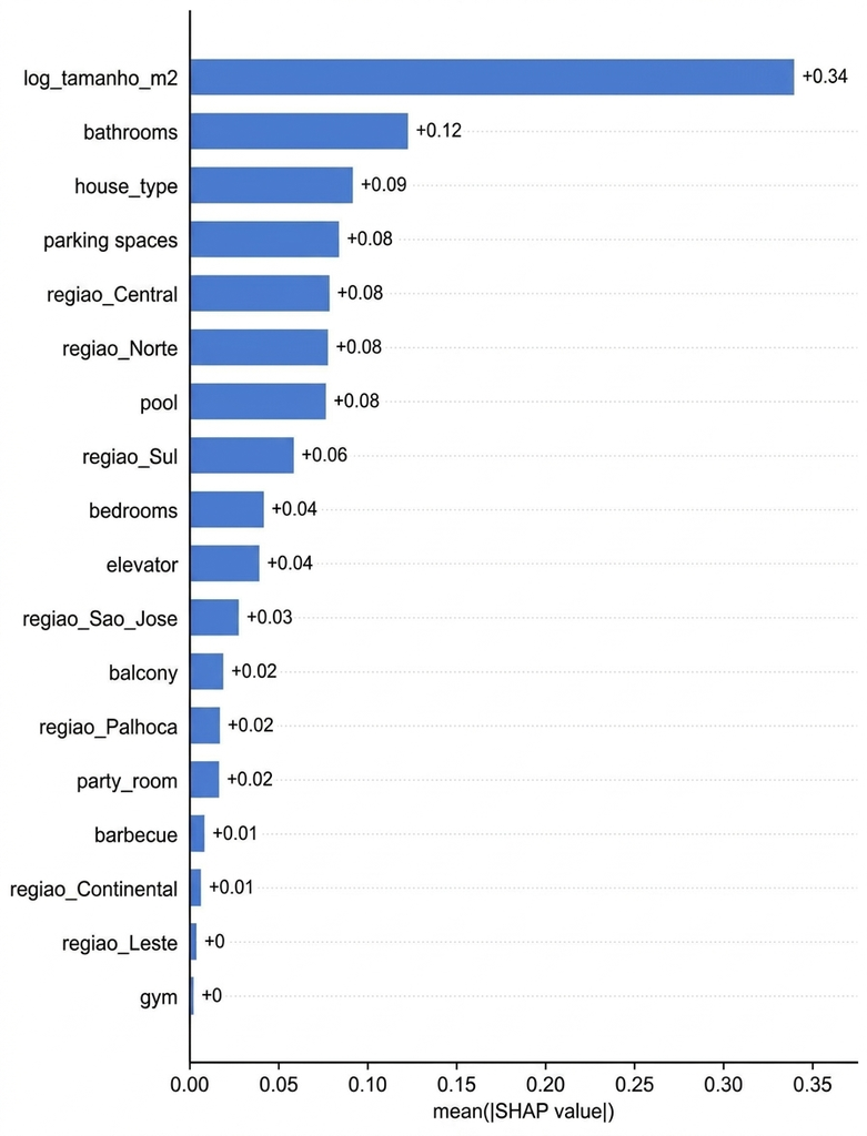
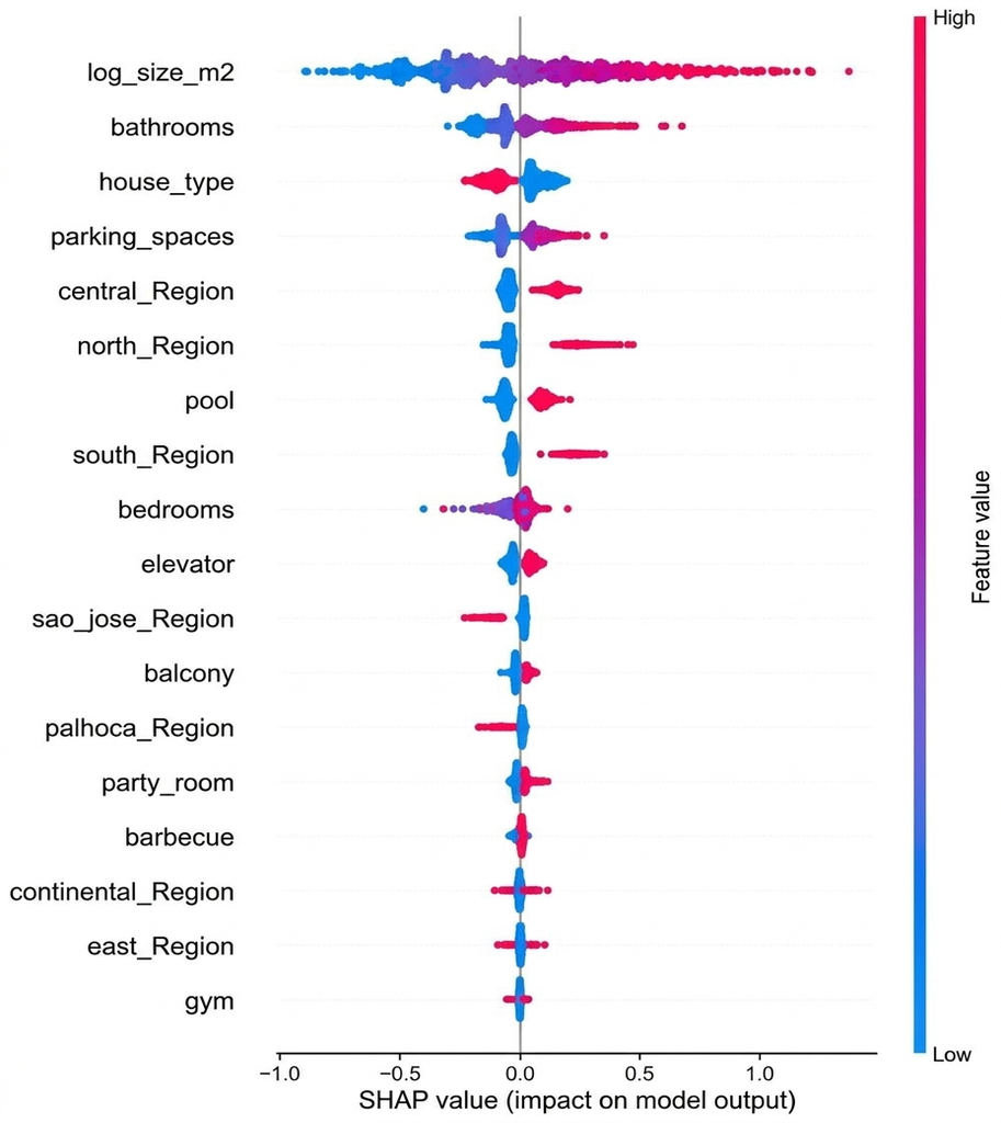
The interpretation of the ensemble models was performed using SHAP values (SHapley Additive exPlanations), a method based on cooperative game theory that assigns to each variable its average marginal contribution to the prediction of each observation (Lundberg and Lee, 2017). SHAP values were calculated on a random sample of 1,000 observations from the test set, applied to XGBoost due to its overall best performance.
Figure 12 presents the ranking of average absolute importance of the variables and Figure 13 presents the beeswarm plot, where each point represents an observation, the horizontal axis indicates the magnitude and direction of the effect of each variable on the prediction, and the color indicates the value of the variable (red = high, blue = low).
Figure 12. Mean absolute importance of variables — SHAP values (XGBoost)
Source: Original survey data
Figure 13. Impact of variables on the predicted price — SHAP values (XGBoost)
Source: Original survey data
The variable with the highest SHAP importance was log_tamanho_m2, followed by regional variables, confirming that size and location are the main determinants of real estate value in Greater Florianópolis. The beeswarm confirms that larger properties have higher SHAP values for the size variable, meaning that the larger the property, the greater its contribution to increasing the predicted price. This pattern is consistent with the elasticity estimated by OLS, but XGBoost captures this relationship more flexibly, without restricting it to a fixed proportion between size and price. Regional variables show high magnitude effects, reflecting the strong geographic component in determining real estate prices, a result widely documented in hedonic literature since Rosen (1974). The comparison between the ordering of importance of OLS coefficients and the SHAP values of XGBoost reveals convergence, as in both methods, size, location, and number of bathrooms are among the main determinants of value.
Market segment analysis
As a complementary analysis, the three models were re-estimated on a subset of the database limited to the closed interval between the 5th percentile and the 95th percentile of the value distribution (R$ 350,000 to R$ 4,712,500), corresponding to 7,268 observations (90.2% of the total). The objective was to verify whether the predictive performance of the models improves when properties at the extremes of the distribution (whose value is determined by factors not captured by the available variables, such as high standard or some irregularity) are excluded from the scope. Table 8 presents the comparison between the two subsets.
Table 8. Performance of the models: full database vs segment [p5-p95]
| Model | To clip (the shapefile) | R² | RMSE | MAPE |
|---|---|---|---|---|
| OLS | Complete | 0,7168 | 971.153 | 29,17% |
| OLS | Segmented | 0,5809 | 600.663 | 27,27% |
| Random Forest | Complete | 0,7339 | 941.302 | 25,69% |
| Random Forest | Segmented | 0,7165 | 494.002 | 23,78% |
| XGBoost | Complete | 0,7419 | 927.113 | 26,27% |
| XGBoost | Segmented | 0,7213 | 489.794 | 23,69% |
Source: Original research results
The most relevant result of this analysis is the sharp drop in the OLS R² when removing outliers (from 0.717 to 0.581, a reduction of 13.6 percentage points), in contrast to the stability of the ensemble models, whose R² dropped only 1.7 and 2.1 percentage points for Random Forest and XGBoost, respectively. This pattern has a statistical explanation: R² is defined as the proportion of total variance explained by the model, and properties at the extremes of the distribution amplify this total variance. By removing them, the total variance drops substantially, and the OLS, being a global model that estimates unique coefficients for the entire sample, loses both the variance that supported its R² and the influential observations that calibrated its coefficients. Tree-based models, by performing local data partitioning, are structurally independent of this influence, a result consistent with the documented robustness of ensemble methods to influential observations (Breiman, 2001).
The improvement in MAPE in the segment was more modest for all models (between 1.9 and 2.6 percentage points), indicating that the unexplained variance is distributed across the entire price range and not concentrated at the extremes. This information suggests that the predictive limitation of the models is structural, determined by the absence of relevant variables in the listing data (such as condition, finish quality, and floor), and cannot be simplified by sample cuts or alternative methodological choices. This result reinforces the recommendation for the use of ensemble models for hedonic pricing in heterogeneous markets, where the presence of atypical properties is inevitable and the performance of OLS may be overestimated when evaluated on the complete sample.
In summary, this study analyzed the efficiency of machine learning techniques in the hedonic pricing of residential properties in Greater Florianópolis. The XGBoost model presented the best overall predictive performance, with an R² of 0.742 and an RMSE of R$ 927,113, outperforming Random Forest and OLS. Random Forest achieved the lowest relative error (MAPE = 25.69%), indicating greater accuracy for intermediate-value properties. The most relevant attributes in price formation, both by OLS coefficients and XGBoost SHAP values, were property area, location region, and number of bathrooms. Implicit regional premiums were significant, with properties in the North region of Florianópolis being 111% more valuable than equivalent properties in Biguaçu, and those in the South region, 105% more valuable. Among amenities, a pool (+20%) and an elevator (+13%) showed the highest implicit premiums. The market segment analysis demonstrated that OLS depends on properties at the extremes of the distribution to sustain its global fit, while tree-based models maintained stable performance, highlighting the superiority of ensemble methods for pricing applications in heterogeneous markets. However, the data comes from online advertisements, reflecting the asking price and not the effectively transacted price, which may introduce an overestimation bias. Relevant variables for price determination are not available in the advertisements (such as condition, floor, solar orientation, view, and quality of finishes), which limits the predictive power of the models and explains the residual MAPE of approximately 25%. The sample corresponds to a single temporal snapshot (March 2026), not allowing for analysis of market trends or seasonality.
4. Conclusion
The study aimed to analyze the efficiency of machine learning techniques in the hedonic pricing of residential properties in the Greater Florianópolis region, using data collected via web scraping from online real estate portals. It was found that XGBoost presented the best overall predictive performance, with an R² of 0.742 and an RMSE of R$ 927,113, while Random Forest achieved the lowest relative error, with a MAPE of 25.69%, outperforming OLS in all evaluated metrics. The main price determinants identified were the property’s built area, location region, and the number of bathrooms, with significant regional premiums, such as that of the North region of Florianópolis, which was worth 111% more than equivalent properties in Biguaçu. Among the amenities, swimming pool and elevator registered the highest implicit premiums. The study’s main contribution lies in demonstrating the robustness and superiority of ensemble methods for hedonic pricing in heterogeneous real estate markets, where the presence of atypical properties is common, offering a more precise tool for buyers, sellers, and investors.
However, the study presents limitations inherent to the nature of the data, which are derived from online advertisements and reflect the asking price, not the transacted price, which may introduce an overestimation bias. The OLS model, in turn, presented severe multicollinearity between the built area and the number of rooms, which restricts the individual interpretation of these variables. Variables relevant to price determination, such as condition, floor, solar orientation, and quality of finishes, were not available in the advertisements, limiting the predictive power of the models and explaining the residual MAPE of approximately 25%. The sample corresponded to a single temporal cut in March 2026, preventing the analysis of trends or seasonality. For future studies, it is suggested to incorporate explicit spatial variables, such as distance to employment hubs and beaches, the use of actual transaction data, and the collection of data over a broader temporal period to model price dynamics and the impact of economic cycles.
Bibliographic References
Breiman, Leo. 2001. Random Forests. Machine Learning 45(1): 5-32.
Campos, R. B. A. 2017. O mercado imobiliário residencial no município de São Paulo: uma abordagem de preços hedônicos espacial. Nova Economia 27(1): 303–337.
Chen, Tianqi; Guestrin, Carlos. 2016. XGBoost: A Scalable Tree Boosting System. Proceedings of the 22nd ACM SIGKDD International Conference on Knowledge Discovery and Data Mining
Dantas, Rubens Alves; Magalhães, André Matos; Vergolino, José Raimundo de Oliveira. 2007. Avaliação de imóveis: a importância dos vizinhos no caso de Recife. Revista de Economia Aplicada, Ribeirão Preto, v. 11, n. 2, p. 231-251, abr./jun
Field, Andy. 2018. Discovering Statistics Using IBM SPSS Statistics. 5ª ed. Londres: SAGE Publications.
Florianópolis. 2023. Lei Complementar N. 739, de 04 de maio de 2023. Altera a Lei Complementar N. 482, de 2014 (Plano diretor de Florianópolis) e consolida seu processo de revisão. Art. 210. Disponível em: https://www.cmf.sc.gov.br/proposicoes/Leis-Complementares/2023/1/0/89810. Acesso em 20 mar. 2026.
Fundação Instituto de Pesquisas Econômicas [FIPE] – Índice Fipezap venda residencial, informe de 12/2024. Disponível em https://downloads.fipe.org.br/indices/fipezap/fipezap-202412-residencial-venda-publico.pdf. Acesso em 20 mar. 2026.
Fávero, L. P. 2003. Modelos de preços hedônicos aplicados a imóveis residenciais em lançamento no município de São Paulo. Working Paper n. 03/002. FEA-USP, São Paulo.
Fávero, L. P.; Belfiore, P.; Lima, G. A. S. 2008. Modelos de precificação hedônica de imóveis residenciais na região metropolitana de São Paulo: uma abordagem sob as perspectivas da demanda e da oferta. Estudos Econômicos (São Paulo) 38(1).
Fávero, L.P.; Belfiore, P. 2024. Manual de Análise de Dados: estatística e Machine Learning com EXCEL®, SPSS®, STATA®, R® e Python®. 2ed. LTC, Rio de Janeiro, RJ, Brasil
Goodman, Allen C.; Thibodeau, Thomas G. 1995. Age-related heteroskedasticity in hedonic house price equations. Journal of Housing Research 6(1): 25–42.
Instituto Brasileiro de Geografia e Estatística [IBGE]. 2023. Panorama do Censo 2022. Disponível em https://censo2022.ibge.gov.br/panorama/. Acesso em 20 mar. 2026.
Kappel, M. A. A.; Teodoro, L. A. 2021. Modelo Hedônico para Estimação do Valor de Imóveis: Aplicação em Nova Friburgo-RJ. VETOR — Revista de Ciências Exatas e Engenharias 30(1): 28-37.
Lundberg, Scott M.; Lee, Su-In. 2017. A unified approach to interpreting model predictions. Advances in Neural Information Processing Systems 30: 4765–4774.
Malpezzi, Stephen. 2003. Hedonic pricing models: a selective and applied review. In: O’Sullivan, Tony; Gibb, Kenneth (Eds.). Housing Economics and Public Policy: Essays in Honor of Duncan Maclennan. Oxford: Blackwell Science, p. 67-89
Moro, Matheus Fernando. 2017. Modelo híbrido de séries temporais para previsão de demanda do mercado imobiliário de São Paulo. Tese (Doutorado).
Pedersen, Anne Marie B.; Weissensteiner, Alex; Poulsen, Rolf. 2013. Financial planning for young households. Annals of Operations Research 205: 55–76
Rosen, S. 1974. Hedonic prices and implicit markets: product differentiation in pure competition. Journal of Political Economy 82(1): 34–55.
Sirmans, G. Stacy; Macpherson, David A.; Zietz, Emily N. 2005. The composition of hedonic pricing models. Journal of Real Estate Literature 13(1): 1–44.
Article originating from the Course Conclusion Work of the Specialization in Data Science and Analytics of the MBA USP/Esalq
To learn more about the course, click here and access the MBX Academy platform