Article

Pablo Diego de Albuquerque Pereira; Diego Pedroso dos Santos

DOI: 10.22167/2675-6528-202602302

Article derived from a Final Course Work (TCC), with content based on the student’s original work and adapted to the editorial format of the Revista E&S with the support of the ResumeAI tool, an artificial intelligence solution developed by the Pecege Institute for textual synthesis and organization.

Summary

Statistical arbitrage via Pairs Trading is a consolidated strategy in quantitative portfolio management. The application of unsupervised Machine Learning for asset pair selection was investigated, comparing its performance with the classic Cointegration approach in the Brazilian financial market. Historical data from B3, from 2004 to 2025, were collected and processed by walk-forward validation. The Machine Learning methodology combined Principal Component Analysis (PCA) and the DBSCAN algorithm to identify asset clusters, while the Baseline approach used classic sector Cointegration. Welch’s T-test and Levene’s test were applied for statistical inference. The results indicated that, although the difference in average daily returns was not statistically significant (p = 0.656), the Machine Learning strategy achieved a superior cumulative return (202.48% vs. 157.24%) and lower annualized volatility (4.29% vs. 4.62%) compared to the Baseline. Levene’s Test suggested a trend of risk reduction (p = 0.066) by the Machine Learning approach. It was concluded that the Machine Learning pipeline improved the quality of the selected pairs, resulting in a portfolio with lower volatility and higher cumulative return over long horizons, without necessarily predicting superior returns in daily statistical terms.

Keywords: Clustering Algorithms; Principal Component Analysis; B3; Cointegration; Quantitative Finance.

1. Introduction

The evolution of financial markets in recent decades has consolidated the adoption of quantitative strategies as a central tool for institutional portfolio management. Among the various types of systematic operations, statistical arbitrage stands out for exploiting temporary pricing deviations between historically correlated assets, based on the premise of mean reversion. This approach, known as “Pairs Trading”, was popularized in the 1980s by Morgan Stanley analysts and has since become one of the most studied “hedge fund” strategies in academic literature (Gatev; Goetzmann; Rouwenhorst, 2006).

The operational principle of “Pairs Trading” is relatively intuitive: a pair of assets whose prices exhibit a common long-term trajectory is identified, and short-term divergences are traded by buying the relatively depreciated asset and short-selling the relatively overvalued one. When prices converge to their historical equilibrium, both positions are closed with profit. This dynamic constitutes a “market neutral” strategy, as directional market exposure is theoretically neutralized by the combination of long and short positions, a characteristic particularly valued in scenarios of high macroeconomic uncertainty.

Historically, pair selection has been based on fundamentalist criteria, especially sector classification. It is presumed that companies from the same economic segment are subject to similar systemic risks and, therefore, present a higher probability of cointegration. However, such a heuristic faces evident structural limitations in the Brazilian market. B3, the country’s main stock exchange, is characterized by high sector concentration, with the commodities and financial segments accounting for a substantial share of total capitalization and trading volume. This asymmetry makes it difficult to construct diversified portfolios based exclusively on the sector criterion, reducing the universe of viable pairs and potentially leading to the formation of suboptimal portfolios. Additionally, sector classification is static and does not always capture latent price dynamics, which can compromise the co-movement premise, especially during stress periods (Caldeira, 2013).

In the context of increasing availability of data and computational power, unsupervised Machine Learning techniques emerge as a promising alternative. Instead of relying exclusively on rigid a priori categorizations, algorithms such as DBSCAN (“Density-Based Spatial Clustering of Applications with Noise”), combined with Principal Component Analysis (PCA), allow for the construction of a hybrid model. In this architecture, empirical similarity based on latent price dynamics, mathematically extracted via PCA, acts by breaking down sectoral barriers, enabling the identification of atypical co-movements and pairs of high intersectoral cointegration. The precedence of the combination between PCA and DBSCAN was demonstrated by Sohail et al. (2020), obtaining a significant advantage over purely categorical approaches.

The literature on “Pairs Trading” in the Brazilian market remains relatively scarce when compared to international production, especially regarding the application of Machine Learning techniques. This study partially fills this gap, reporting empirical evidence from twenty-one years of historical data, and validates the generalization of Sohail et al.’s (2020) framework in a distinct emerging market. The identification of robust pairs meets the direct interest of quantitative managers seeking uncorrelated alpha, as, during severe systemic crises, hybrid Machine Learning modeling stands out for its adaptability in finding empirically validated co-movements crossing sectoral conventions. Thus, the general objective of this work is to develop and evaluate an unsupervised Machine Learning model for asset selection in “Pairs Trading” strategies, comparing its performance with the traditional Classical Cointegration approach in the Brazilian financial market, in the period from 2004 to 2025.

2. Material and Methods

Regarding ethical aspects, the study falls within the exceptions provided by the institution’s Manual of Norms (item 5.2) and by CNS Resolution No. 510, of 2016, Art. 1º, Sole Paragraph, Items II and III. This is because it only uses publicly accessible and public domain information from the financial market, not involving the direct or indirect participation of human beings or the handling of sensitive data, thus being exempt from review by the Research Ethics Committee (CEP).

This study was limited to the Brazilian stock market (B3), using the universe of assets that are part of or have historically been part of the Bovespa Index (IBOV) in the period from 2004 to 2025. Other asset classes (derivatives, ETFs, real estate funds) and international markets were not considered. The simulation model did not incorporate transaction costs (brokerage fees, emoluments, and stock lending costs – BTC), adopting as a premise execution at closing prices without market impact. The methodological flow and logical structure of the study are presented in Figure 1.

Figure 1. Methodological Flow and Logical Structure of the Study.

Source: Original survey data.

The data were collected via the unofficial tvDatafeed (v2.0+) Python library, which accesses historical data from the TradingView platform for the BMFBOVESPA (B3) exchange. The study universe comprised approximately 100 IBOV assets over the analyzed period. For each asset, daily closing prices (close) series were obtained, totaling about 5,000 bars per asset. The files were saved in CSV format and subsequently consolidated into a single “Parquet” file via a preprocessing pipeline. The IBOV index, used as an external “benchmark” in the comparative analysis, was collected separately via the public yfinance API.

The following eligibility criteria were applied to the initial universe to ensure liquidity and data quality, as shown in Table 1.

Table 1. Operational parameters

Criterion	Parameter
Daily minimum volume	Average > R$ 1 million in the training period
Data availability	Minimum of 252 continuous trading days of history
Continuity	Absence of gaps greater than 5 consecutive trading days
Quality	Absence of negative values or price outliers (>3σ)

Source: Original source

Assets that did not meet such criteria were excluded from the selection universe in each “walk-forward” training window.

The raw data were submitted to a standardized treatment pipeline, which included: 1. Cleaning: Removal of trading days with missing data (NaN) and treatment of “splits” not adjusted to the API; 2. Logarithmic returns: Closing prices were converted into log-returns, according to Equation (6):

r_t = ln(P_t / P_t-1) (6)

3. Z-Score Normalization: The returns matrix was normalized (zero mean, unit standard deviation) per variable (asset) before applying PCA; 4. Consolidation: The processed data were saved in “Parquet” format.

The existence of survivorship bias is recognized, as the universe of assets is based on the historical composition of IBOV as available in the data source. Such a limitation is common to academic “backtesting” studies and is partially mitigated by the focus on high-liquidity assets.

The implementation was developed entirely in Python 3.10, structured in three sequential Jupyter “notebooks”. The computational ecosystem was based on the libraries pandas, numpy, scikit-learn, statsmodels, scipy, duckdb, tvdatafeed, and yfinance.

To simulate the operation in a real environment and ensure methodological rigor, the “Walk-Forward” validation protocol was adopted, with training windows of 12 months and testing windows of 6 months, advancing in semi-annual steps throughout the entire historical horizon (January 2004 to December 2025). The DBSCAN parameters ɛ and min_samples were fixed at 0.30 and 3, respectively, without iterative calibration via Distance Heuristic, due to computational cost and inter-window instability.

Two pair selection approaches were compared. In the Baseline approach (Classical Cointegration), pairs were formed exclusively between assets from the same economic sector (as listed on the B3 website). For each candidate pair, the cointegration hypothesis was tested using the two-step Engle-Granger procedure. Pairs with p-value ≤ 0.05 were considered eligible for trading in the following window.

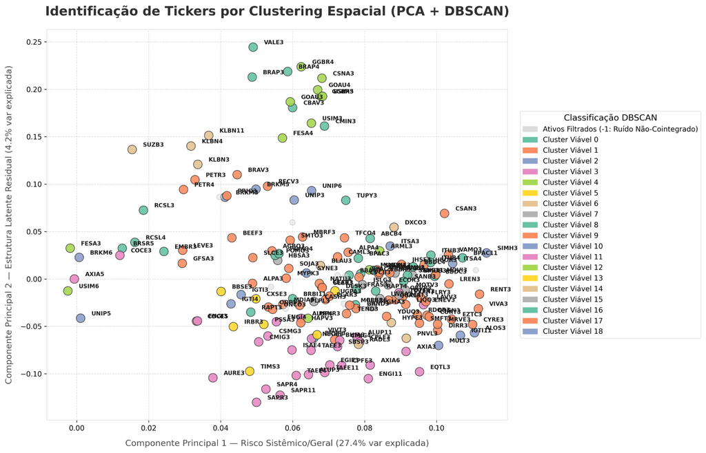
The proposed approach (Machine Learning – ML) was based on the “framework” by Sohail et al. (2020), adapted to the Brazilian market and operationalized in a pipeline integrated by a “walk-forward” window. The matrix of logarithmic returns was normalized via Z-Score per asset, followed by the application of Principal Component Analysis (PCA) for the retention of the four components with the highest expressiveness. The resulting scores were concatenated with binary (“dummy”) variables representing the economic sectors of B3. On this hybrid representation, the DBSCAN algorithm (eps = 0.30; min_samples = 3) was applied, allowing the identification of “clusters” based on empirical similarity and the automatic discarding of noisy assets. Finally, the pairs formed within each grouping were statistically validated by the Engle-Granger Cointegration Test, limiting the final selection to relationships with p-value ≤ 0.05, as illustrated in Figure 2.

Figure 2. Hybrid Identification of “Clusters” in PCA-Dummies Space.

Source: Original survey data.

For both approaches, the “Pairs Trading” strategy implemented followed the classic mean reversion model, operating the normalized “spread” (Z-Score) between the pair’s assets. The “spread” (7) was defined as the residual of the OLS regression between the asset prices:

Spread_t = P_dep,t – β. P_ind,t (7)

where β (hedge ratio) was estimated via OLS in the formation period. The Z-Score (8) of the “spread” was calculated in a rolling window of 60 trading days:

Z_t = (Spread_t – μ₆₀) / σ₆₀ (8)

The operational parameters of the operations are presented in Table 2.

Table 2. Input and output parameters

Event	Condition	Action
Long “input”	Z < -2.0	Buy dependent asset, sell independent asset
Short “input”	Z > +2.0	Sell dependent asset, buy independent asset
Natural Output	Z ≥ 0.0 (“Long”) or Z ≤ 0.0 (“Short”)	Closing of position with profit/loss
Forced output	End of operation window	Position closed at the price of the last trading session of the window

Source: Original survey data.

The exit threshold adopted was Z = 0.0 (return to equilibrium), with no buffer zone. Positions not closed by the end of the operating window were compulsorily liquidated on the window’s closing date.

The portfolio simulation was developed chronologically and consolidated (all pairs in a single time series), with the parameters shown in Table 3.

Table 3. Financial parameters

Parameter	Value
Initial Capital	USD 100,000.00
Trade allocation	10% of available capital
Maximum leverage	1:1 (no leverage)
Max. simultaneous positions per asset	2
Transaction costs	Unmodeled (documented limitation)

Source: Original survey data.

At each trading session, the portfolio value was updated by summing the P&L (“profit and loss”) of all open positions. The daily return (9) of the portfolio is:

R_portfolio,t = (V_t – V_t-1) / V_t-1 (9)

where V_t represents the total portfolio value on trading day t.

The strategies were compared by the following metrics, listed in Table 4, calculated on the resulting capital curve.

Table 4. Metrics and Indicators

Metric	Definition
Total Return	(Vfinal – Vinitial)/Vinitial
Annualized return	(1 + Rtotal)^(1/n) – 1, where n = years
Annualized Volatility	σdaily × √252
Sharpe Ratio	daily / daily × √252
Alpha vs. IBOV	Total Return Strategy – Total IBOV Return

Source: Original source

To verify if the observed performance differences are statistically robust, two tests were applied: Welch’s T-test, which assesses the significance of the difference between the means of the daily returns of the two strategies (null hypothesis: the means are equal), and Levene’s Test, which assesses whether the variances (and risks) of the strategies differ significantly (null hypothesis: the variances are equal). Both were applied with a significance level of 5% (α = 0.05).

3. Results and Discussion

This section presents the results of the comparison between the Pairs Trading strategies — Baseline (Classical Cointegration) and Machine Learning (PCA + DBSCAN) — for the period from 2004 to 2025. The findings are organized into comparative performance, statistical inference, and comparison with the market benchmark (IBOV), discussing their implications and limitations.

Comparative Performance

Table 5 summarizes the performance metrics of both strategies.

Table 5. Performance comparison: ML vs. Baseline. Period: 2004–2025.

Metric	Reference point	ML	Δ
Total Return	157,24%	202,48%	+45.24 p.p.
Annualized return	3,14%	3,65%	+0.51 p.p.
Annualized Volatility	4,62%	4,29%	-0.33 p.p.
Maximum Drawdown	-10,01%	-8,18%	+1.83 p.p.
Sharpe Ratio	0,68	0,85	+0,17
Sortino Index	0,10	0,14	+0,04
Daily Average Return	0,0125%	0,0145%	+0.0020 p.p.

Source: Original research results.

The results indicated superior performance of the ML strategy across all evaluated metrics. The accumulated return of ML was 202.48% (annualized at 3.65%), surpassing the Baseline (157.24%, annualized at 3.14%) by 45.24 percentage points over 21 years. In terms of risk, the ML strategy showed reduced annualized volatility (4.29% vs. 4.62%) and mitigated maximum Drawdown (-8.18% vs. -10.01%). These improvements resulted in a gain in risk-adjusted return metrics, with the Sharpe Ratio of 0.85 (vs. 0.68) and the Sortino Ratio of 0.14 (vs. 0.10), suggesting that the selection via clustering generated a portfolio with a more stable spread and lower exposure to market tail risk.

Equity Curve(“Equity Curve”)

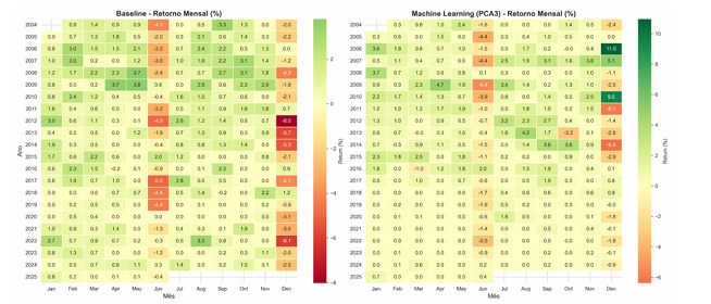
The capital curves of both strategies showed consistent growth. The ML strategy’s trajectory presented a slightly superior slope, with a difference that accumulated progressively, consistent with the 0.002% difference in daily average return. Both curves confirmed the market-neutral nature of the strategies, without significant drawdowns during periods of systemic crisis (Subprime 2008, Brazilian Recession 2015-2016, Pandemic 2020), unlike directional strategies, according to Figure 3.

Figure 3. Capital Curve Evolution: Baseline vs. “Machine Learning”.

Source: Original research results.

Risk Profile

The annualized volatility of 4.62% (Baseline) and 4.29% (ML), and the limited maximum drawdowns (-10.01% and -8.18%, respectively), were drastically lower than the historical volatility of IBOV (~25% per year). This risk profile is a central characteristic of long/short strategies. In the universe of market-neutral strategies, volatilities below 5% per year are compatible with long-term fixed-income products, indicating CDI as a more suitable benchmark than IBOV. Both strategies demonstrated the ability to generate alpha over the low-risk cost of capital, with the ML approach optimizing the risk-return profile through the Machine Learning filter (PCA and DBSCAN).

Statistical Inference

To verify the statistical robustness of the performance differences, independent tests were applied to the daily return series of the consolidated portfolio.

Welch’s T-test — Comparison of Mean Returns

Welch’s T-test assessed the null hypothesis that the difference between the mean daily returns of the two strategies is zero. Table 6 presents the results.

Table 6. ML x Baseline average return results

Statistics	Value
Average daily return — ML	0,0145%
Average daily return — Baseline	0,0125%
t-value	0,4448
P-Value	0,6565
Conclusion	Do not reject Ho

Source: Original research results.

With a p-value of 0.6565, higher than the 5% significance level, there was insufficient statistical evidence to state that the average returns differ. The 0.002% difference in average daily return can be attributed to random market variation, rather than to a structural superiority of the algorithm.

Levene test — Comparison of Volatilities

Levene’s Test assessed whether the variances of the two strategies differed significantly. The results are presented in Table 7.

Table 7. ML x Baseline volatility results

Statistics	Value
Annualized volatility — ML	4,29%
Annualized volatility — Baseline	4,62%
Levene’s statistic
P-Value	0,0659

Source: Original research results.

The p-value of 0.0659, marginally above 0.05, suggests a trend towards risk reduction by the ML approach, consistent with the lower volatility observed numerically. In financial studies with long series, p-values between 0.05 and 0.10 are often considered marginally significant (FIELD, 2018), requiring caution in interpretation.

Comparison with Market Benchmark (IBOV)

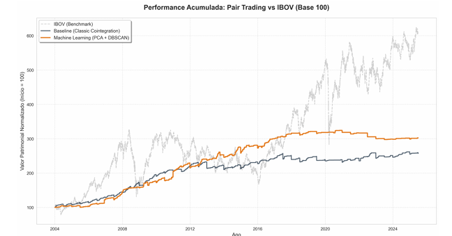
The IBOV accumulated a return of 509.78% in the period from 2004 to 2025. However, direct comparison with the IBOV is methodologically inadequate, as directional strategies like the IBOV have a beta close to 1, while the long/short strategies of this study operate with a beta close to zero, eliminating directional exposure. The most relevant comparison would be the Alpha generated over the low-risk opportunity cost (CDI), which extrapolates the scope of this study. The nominal Alpha calculated for the Baseline was -352.54% and for the ML was -307.30%, reflecting the cost of market neutrality: the renunciation of directional market return in exchange for significantly lower risk and almost zero correlation with the index, as illustrated in Figure 4.

Figure 4. Accumulated Performance: “Pair Trading” vs. IBOV (Base 100).

Source: Original research results.

Synthetic Analysis of Transactional Break-Even

Although the backtest was ideally parameterized (frictionless), the robustness of the profit differential (+45.24 p.p.) of the ML strategy required modeling friction costs. The calculation of the break-even spread, considering the final gross balance of the ML portfolio in relation to the net excess generated above the Baseline, indicated that the cross-sectional break-even point requires consolidated transactional costs higher than 0.47% per month per traded pair. This parametric ceiling of 0.47% p.m. accommodates Brazilian average institutional fees (Brokerage flat + B3 Fees ≈ 0.03% entry/exit) and moderate stock lending premiums (average historical BTC rate in the range of 2% to 4% per year, or ~0.15% to 0.30% per month). This margin differential proves the operational feasibility of the DBSCAN logic in hedge funds, indicating that the observed superiority is not compromised by trivial local market slippages.

Sensitivity Analysis of Parameters

Impact of the Number of PCA Components

The retention of 4 main components, which explain approximately 74.5% of the variance, was the configuration that best balanced representational richness and computational efficiency. Tests with 2 components (about 61% of the variance) resulted in lower clustering quality, with higher intra-cluster entropy, as evidenced by the reduction in the Silhouette Index.

Time Stop Sensitivity

The Time Stop parameter, defined in 20 trading days, was empirically calibrated on the training data. Positions that do not converge within this period tend to be trending pairs, i.e., pairs whose cointegration has broken down. Forced closure is an essential risk management rule to avoid unlimited losses in positions without mean reversion.

Limitations of the Results

The following limitations should be considered when interpreting the results:

Absence of transaction costs: The model did not include brokerage fees, B3 emoluments, or stock lending costs (BTC) for short operations. Under real conditions, returns would be lower, potentially impacting the relative comparison between strategies.

Survivorship bias: The universe of assets, based on historical compositions available via API, may introduce an optimistic bias by not including delisted or incorporated assets.

Slippage and market impact: The premise of execution at closing prices disregards the depth of the book and the impact of larger magnitude orders.

Walk-Forward Lookback: Although the walk-forward protocol eliminates lookahead bias, the 12-month window for training may be insufficient to capture longer-duration structural market regimes.

In summary, this study demonstrated that the application of unsupervised Machine Learning for pair selection in Pairs Trading represents a viable alternative to Classical Cointegration in the Brazilian market. The combination of PCA and DBSCAN, operationalized via a walk-forward protocol, identified groups of assets with related price dynamics that transcend sectoral boundaries. The main finding was the superiority in accumulated return (+45.24 p.p.) of the ML strategy, without compromising the risk profile and with a tendency to reduce volatility. This positions the ML approach as a methodological evolution compared to the sectoral heuristic, even without formal statistical significance in the comparison of average daily returns. This difference, real and economically relevant, is attributed to the improvement in the quality of pair selection, and not to return prediction, which is consistent with the theory of efficient markets.

4. Conclusion

This study sought to develop and evaluate an unsupervised Machine Learning model for asset selection in Pairs Trading strategies, comparing its performance with the traditional Classical Cointegration approach in the Brazilian financial market, during the period from 2004 to 2025. It was found that the Machine Learning-based strategy, which combined Principal Component Analysis (PCA) and the DBSCAN algorithm, generated a superior cumulative return of 202.48% compared to 157.24% from the Baseline approach. A reduction in annualized volatility to 4.29% against 4.62% from the Baseline was also observed, along with a mitigated maximum drawdown. Although Welch’s T-test did not indicate a statistically significant difference in daily average returns (p = 0.656), Levene’s test suggested a trend towards risk reduction (p = 0.066) by the Machine Learning approach. Both strategies demonstrated a market-neutral character, with annual volatilities significantly lower than that of the IBOV. The main practical contribution lies in the improvement of the quality of selected pairs, which translated into a portfolio with a superior risk-return profile, delivering higher returns with lower volatility over long horizons, without necessarily predicting superior daily statistical returns. This finding reinforces the applicability of the framework in an emerging market like Brazil.

However, the interpretation of the results must consider some limitations, such as the absence of transaction costs in the model, the survival bias of assets, and the assumption of execution without slippage or market impact. Additionally, the walk-forward protocol’s lookback window may be insufficient to capture longer-duration market regimes, and the model did not incorporate regime switching mechanisms. For future studies, it is suggested to incorporate real BTC costs, apply Deep Learning techniques to model non-linearities and cointegration breaks, use Reinforcement Learning for dynamic order calibration, evaluate the strategy with intraday data, and integrate fundamental filters in a quantamental approach.

Bibliographic References

Caldeira, J.F. 2013. Seleção de carteiras utilizando o modelo Fama-French-Carhart. Brazilian Review of Finance 11(2): 173-198.

Field, A. 2018. Discovering Statistics using IBM SPSS Statistics. 5ed. SAGE Publications, London, Inglaterra, UK.

Gatev, E.; Goetzmann, W.N.; Rouwenhorst, K.G. 2006. Pairs trading: performance of a relative-value arbitrage rule. The Review of Financial Studies 19(3): 797-827.

Resolução CNS nº 510, 2016 [Referência completa não encontrada no documento original]

Sohail, A.; et al. 2020. Pairs trading in the Chinese stock market: new evidence from DBSCAN clustering. International Journal of Finance & Economics 27(2): 1-20.

Article originating from the Course Conclusion Work of the Specialization in Data Science and Analytics of the MBA USP/Esalq

To learn more about the course, click here and access the MBX Academy platform