Nowcasting and Return and Risk Forecast of the Tesouro Direto Ipca+ by Market Regime

Silva, Gledson Duarte da; Barbosa, William

doi:10.22167/2675-6528-202602223

Article

September 15, 2026

Nowcasting and Return and Risk Forecast of the Tesouro Direto Ipca+ by Market Regime

Gledson Duarte da Silva; William Barbosa

DOI: 10.22167/2675-6528-202602223

Article derived from a Final Course Work (TCC), with content based on the student’s original work and adapted to the editorial format of the Revista E&S with the support of the ResumeAI tool, an artificial intelligence solution developed by the Pecege Institute for textual synthesis and organization.

Summary

The growing participation of investors in Tesouro Direto and the sensitivity of inflation-indexed bonds to interest rates, expectations, and regime changes make short-term forecasting of their price and risk movements relevant. The study aimed to estimate and evaluate nowcasting models for the return and risk of Tesouro Direto bonds, focusing on Tesouro IPCA+, considering different market arrangements and seeking evidence on how inflationary shocks, expectations, and regimes affect prices and profitability. To this end, a database was built with prices and rates from Tesouro Transparente, Selic, and IPCA from the Central Bank, using ANBIMA curves as an auxiliary source due to limited historical coverage. Daily logarithmic return, realized volatility over 21 trading days, five-fold temporal validation, comparison between LightGBM and a persistence model, and descriptive use of HMM with two states were employed. The results showed that the return at t+1 oscillated around zero and admitted moderate predictive gain with LightGBM, which outperformed the benchmark model. The risk at t+1 exhibited strong persistence, being better predicted by repeating the most recent value. The findings indicated that return and risk require distinct treatments and that the temporal heterogeneity of the sample is relevant for the economic interpretation of Tesouro IPCA+. The limited coverage of ANBIMA curves restricted the broader incorporation of the interest rate term structure into the main predictive block.

Keywords: Gradient boosting; Hidden Markov Models; Implied inflation; Selic rate; Realized volatility.

1. Introduction

Tesouro Direto was established in January 2002 through a partnership between the National Treasury and the Brazilian Clearing and Depository Company (CBLC), currently B3, marking a significant transformation in retail investor access to the public debt market. Before this initiative, the trading of public securities was restricted to large financial institutions and investment funds. The creation of this platform allowed individuals to invest directly in government bonds, eliminating part of the intermediation and reducing transaction costs (Ferreira, 2015). For the government, the program has consolidated itself as an important mechanism for domestic resource mobilization and an instrument of monetary policy (Perlin, 2016).

For the individual investor, Tesouro Direto opened the possibility of accessing fixed-income assets with different remuneration structures, from fixed rates to post-fixed modalities, linked to the basic interest rate (Selic) and indicators such as the Broad Consumer Price Index (IPCA) (Ferreira, 2015). This diversity expands the range of investment strategies, catering to conservative profiles and those seeking inflation protection. In particular, Tesouro IPCA+, which combines a fixed part with inflation adjustment, guarantees the maintenance of purchasing power over time. However, this type of bond is subject to mark-to-market fluctuations, with its value potentially oscillating substantially depending on inflation expectations and current market interest rates (Portal do Investidor [GOV], 2022).

The dynamics between interest rates, inflation behavior, and negotiations in Tesouro Direto reveal important aspects of this market’s microstructure. During periods of Selic rate hikes, as observed in the monetary tightening cycles of 2021-2022 (Banco Central do Brasil [BACEN], 2022), the increase in public debt yields attracts greater demand for post-fixed securities linked to the Selic rate. Comparatively, the appreciation of inflation-indexed bonds, such as Tesouro IPCA+, becomes less significant in the short term due to the increased opportunity cost, although they maintain their appeal as a real store of value during periods of inflationary pressure (Júnior and Tavares, 2024). Inflation in Brazil is historically unstable and subject to domestic and external frictions (Minella et al., 2003), and studies indicate that Brazilian inflationary persistence is high, prolonging disturbances and accentuating risks for investors in inflation-corrected bonds (Silva and Leme, 2008).

The recognition of these distinct market configurations is essential for understanding the fluctuations in the return and risk of Tesouro Direto bonds, directly impacting investor behavior and the pricing of public securities. Tesouro Direto has shown consistent growth in participation, volume, and stock, reinforcing the practical relevance of analyses like this. In December 2024, the number of active investors reached 3,013,921 people, and the program’s bond accumulation closed at R$156.9 billion (Tesouro Nacional [GOV], 2025). In July 2025, the reserve exceeded R$185.7 billion, with inflation-indexed bonds representing approximately 51.2% of this amount (Ministério da Fazenda [GOV], 2025).

In this scenario, short-term forecasting of price and risk movements for inflation-indexed bonds becomes relevant. The concept of nowcasting refers to the immediate update of the estimate for the bond’s next movement (Bańbura, Giannone, and Reichlin, 2010; Corsi, 2009). In mark-to-market assets, new information about interest rates, inflation, and real premiums can rapidly alter price and risk. To address this complexity, modeling can incorporate the idea of market regimes, which represent distinct contexts of return and risk, and can be explored through models such as Hidden Markov Models (Hamilton, 1989; Rabiner, 1989). Furthermore, machine learning techniques, such as LightGBM, are suitable for combining past information non-linearly and generating forecasts (Ke et al., 2017).

The increased participation of investors in Tesouro Direto and the sensitivity of inflation-indexed bonds to interest rates, expectations, and regime changes make short-term forecasting of their price and risk movements relevant. There is a gap in the in-depth understanding of how inflationary shocks, market expectations, and regime changes affect the prices and profitability of these bonds, which justifies the need for tools that enable more informed decisions in volatile economic environments for investors and managers. Thus, this work aims to estimate and evaluate nowcasting models applied to the forecasting of return and risk of Tesouro Direto bonds, focusing on Tesouro IPCA+, considering different market arrangements and seeking evidence on how inflationary shocks, expectations, and regimes affect prices and profitability.

2. Material and Methods

The study is characterized as applied research, quantitative in nature, formulated as a one-step-ahead forecasting problem, using the information available at each date t to estimate what would happen on the next business day (t + 1).

The database was built from official public sources, with daily price and rate history obtained from Tesouro Transparente (2026), reflecting the secondary market for federal public bonds. The study focused on the Tesouro IPCA+ without semi-annual coupons, selecting the bond with the highest coverage and maturity on May 15, 2035, to avoid automatic price changes.

Macroeconomic series, such as daily Selic (series 11) and monthly IPCA (series 433), were obtained from the Central Bank of Brazil [BACEN] Time Series Management System [SGS]. The raw data period was from March 8, 2010, to January 30, 2026. The monthly IPCA was aligned to the daily calendar, and the 12-month accumulated inflation was constructed. Data from the Brazilian Financial and Capital Markets Association [ANBIMA] on the term structure of interest rates were used as an auxiliary source, but their limited coverage (January 28, 2026, to February 4, 2026) prevented their use in the main predictive comparison.

The construction of the targets followed the literature on “nowcasting” and volatility modeling (Bańbura, Giannone and Reichlin, 2010; Corsi, 2009). General equations for return, risk, and targets at t+1 (1):

RET₁ = In (PU) – In (PUt-1)

where: PUţ: is the observed unit price at t; RETț: is the daily logarithmic return.

RISK₁ = $\frac{{1}{n-1} \sum_{i=0}^{n-1} (RET_{t-i} – \overline{RET_n})^2$

where: RISK₁: is the realized volatility in a rolling window of n trading days; RET: is the average of returns in the window of size n; i: indexes the observations of the rolling window.

RETF1.t = RETt+1

where: RETF1,t: projection of the return at t + 1.

RISK1,t = RISKt+1

where: RISCOF1,ť: projection of risk at t + 1.

Eq. (1.0) defines the daily stock return on a logarithmic scale. Eq. (1.1) defines risk as a measure of recent oscillation calculated from the last 21 trading days, which serves as a monthly approximation of price instability. Eq. (1.2) and eq. (1.3) simply shift these series by one day to create the forecast targets.

The supervised block was estimated using LightGBM, a machine learning method for tabular data that combines past information in a non-linear way (Ke et al., 2017). Conceptual approach of the supervised block (2):

Xt = [Z1,t-l1, Z2,t-l2,………,Zk,t-lk]

where: x₁: represents the vector of attributes available at time t, formed by financial and macroeconomic lags.

ŷt = F(xt) = $\sum_{m=1}^{M} v f_m(x_t)$

where: ŷť: represents the target prediction at time t; F (xī): represents the estimated predictive function; M: represents the total number of trees; v: represents the learning rate; fm(xt): represents the m-th interaction tree.

The regime block was modeled separately by a Gaussian Hidden Markov Model [HMM] with two states, used for descriptive characterization of the sample and not as a central input for predictive comparison (Hamilton, 1989; Rabiner, 1989). The conceptualization of the regime block is summarized in equations (3.0) through (3.3). Conceptual approach of the two-state Gaussian HMM (3):

St ∈ {1, 2}

where: St: represents the hidden state at instant t.

P(St = j St-1 = i) = Pij, i,j∈ {1, 2}

where:pij: represents the transition probability from state i to state j.

Yt = [RETD,t, RISCOD,t]

where: yt: represents the observed vector of return and risk.

yt|St = s ~ Ν(μς,Σς)

where: μs represents the mean; ∑5: represents the covariance matrix of state s.

Table 1 summarizes the central variables of the consolidated “dataset”.

Table 1. Definition of variables

Variable	Operational definition	Source	Variable Type
PU	Daily unit price of the selected Treasury IPCA+	Transparent Treasury	numerical explanatory
IPCA RATE	Daily selling rate of the selected security	Transparent Treasury	numerical explanatory
RET_D	Daily logarithmic return of the unit price	Derivative of PU	numerical explanatory
RISK_D	Realized volatility in 21 trading days of RET_D	Derivative of RET_D	numerical explanatory
SELIC	Daily Selic rate, SGS series 11	SGS/BACEN	numerical explanatory
D_SELIC_1	Daily variation of the Selic	SELIC Derivative	numerical explanatory
D_SELIC_5	5-day accumulated variation of the Selic	SELIC Derivative	numerical explanatory
IPCA	Monthly IPCA, SGS 433 series, aligned with the daily calendar	SGS/BACEN	numerical explanatory
IPCA_12M	12-month accumulated inflation	IPCA Derivative	numerical explanatory
RET_F1	Target for return at t+1	Time shift derivative	numerical dependent
RISK_F1	T+1 risk target	Time shift derivative	numerical dependent

Source: Original survey data

The daily return was calculated on a logarithmic scale. Risk was measured by realized volatility in a 21-trading-day rolling window. The RET_F1 and RISCO_F1 targets were obtained by shifting one position forward (‘shift(-1)’), aiming to predict the next business day based on current information (Corsi, 2009; Bańbura et al., 2010).

The predictors for the supervised block included past values (lags 1, 2, and 5) of RET_D, RISCO_D, SELIC, D_SELIC_1, D_SELIC_5, and TAXA_IPCA, in addition to contemporaneous IPCA and IPCA_12M. The monthly IPCA was aligned to the daily calendar using ‘merge_asof’ with direction ‘backward’ (Júnior and Tavares, 2024).

The HMM was adjusted using standardized RET_D and RISCO_D, with two states, up to 250 iterations, tolerance of 10-4, and seven restarts, selecting the model with the highest log-likelihood (Hamilton, 1989; Rabiner, 1989).

The main predictive block, based on LightGBM, used ‘n_estimators = 400’, moderate regularization, and ‘force_col_wise = True’. ‘Early stopping’ was applied during training. For RISCO_F1, the adjustment was performed on the log1p scale, and the final prediction returned to the original scale by expm1 (Ke et al., 2017; Hyndman and Athanasopoulos, 2021).

External validation was performed with ‘TimeSeriesSplit’ in five folds, with ‘gap = 1’ and dynamic test size (maximum between 120 observations and one sixth of the useful sample). The evaluation period was from April 14, 2010, to January 29, 2026 (Hyndman and Athanasopoulos, 2021). Table 2 summarizes this chronological distribution.

Table 2. Chronological distribution of temporal validation folds

Fold	Training until	Test start	End of test
1	2012-11-29	2012-12-03	2015-07-16
2	2015-07-15	2015-07-17	2018-03-07
3	2018-03-06	2018-03-08	2020-10-22
4	2020-10-21	2020-10-23	2023-06-15
5	2023-06-14	2023-06-16	2026-01-29

Source: Original survey data

The evaluation metrics employed were the Mean Absolute Error (MAE) and the Root Mean Squared Error (RMSE), which allow for the assessment of predictive performance (Hodson, 2022). Equations for the MAE and RMSE metrics (4):

MAE = $\frac{{1}{n} \sum_{i=1}^{n} |y_i – \hat{y}_i|$

RMSE = $\sqrt{\frac{{1}{n} \sum_{i=1}^{n} (y_i – \hat{y}_i)^2}$

where: y₁: represents the observed value in observation i; ŷ¡: represents the value in observation i; n: represents the total number of evaluated observations.

3. Results and Discussion

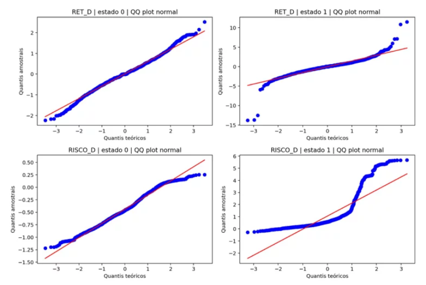
The descriptive analysis of the return (RET_D) and risk (RISCO_D) distributions in each inferred state, presented in Figure 1, revealed approximate compatibility with the normality hypothesis for some configurations. However, the normal probability plots (Figure 2) indicated systematic deviations, suggesting skewness or heavier tails, especially for risk. These findings are descriptive and complementary, without replacing formal normality tests (National Institute of Standards and Technology, 2026).

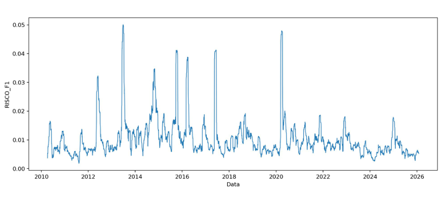
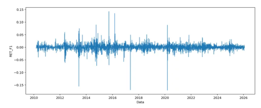
The t+1 return trajectory (RET_F1) showed oscillations around zero throughout the sample, without a clear repetitive pattern, indicating daily instability and strong influence of repricing (Figure 3). In contrast, the t+1 risk dynamics (RISCO_F1) exhibited blocks of higher and lower instability, suggesting stronger short-term continuity (Figure 4). The maximum value of RET_F1 was 0.142691 on 2015-09-24, and the minimum -0.170763 on 2020-03-11. For RISCO_F1, the maximum was 0.050059 on 2013-06-26, and the minimum 0.001813 on 2011-08-09.

Figure 1: Histograms by state with adjusted normal curve

Source: Original survey data

Figure 2: QQ plots by state for RET_D and RISCO_D

Source: Original survey data

Figure 3: Daily return at t+1 out-of-sample

Source: Original survey data

Figure 4: Daily risk at t+1 over the sample

Source: Original survey data

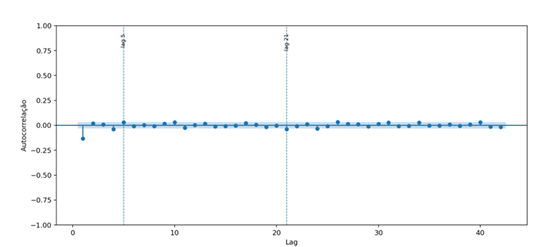
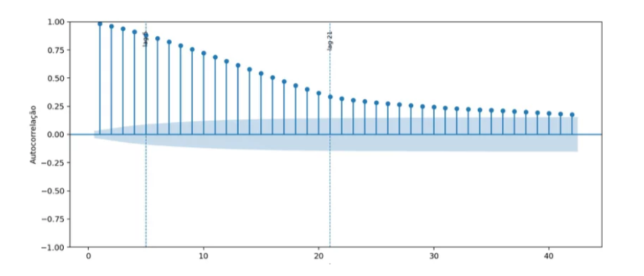
The analysis of the autocorrelation function (ACF) confirmed these differences. For RET_F1, the autocorrelation coefficients were small and without slow decay (Figure 5), although the Ljung Box test still rejected the null hypothesis of white noise (p-value of 1.81 * 10-12), indicating some residual temporal dependence. For RISCO_F1, the ACF showed very high values in the first lags (p1 = 0.983, ρ5 = 0.883, p10 = 0.723, and p21 = 0.337), decreasing gradually (Figure 6). This is consistent with volatility clustering and suggests that periods of instability tend to persist (Hyndman and Athanasopoulos, 2021; Ljung and Box, 1978).

Figure 5: Autocorrelation of return at t+1

Source: Original survey data

Figure 6: Autocorrelation of risk at t+1

Source: Original survey data

The sample heterogeneity was synthesized by descriptive statistics, as in Table 3. The unit price (PU) ranged between 402.270000 and 2389.690000, and the bond rate (TAXA_IPCA) oscillated between 3.010000 and 7.990000. Macroeconomic variables such as monthly IPCA (-0.680000 to 1.620000) and accumulated IPCA over 12 months (1.877488 to 12.131481) also showed significant amplitudes, reflecting distinct monetary and inflationary periods.

Table 3. Definition of the variables

Variable	Minimum	Maximum	Average	Standard Deviation	Observations
PU	402,270000	2389,690000	1338,066352	637,209710	3967
IPCA RATE	3,010000	7,990000	5,673426	1,048831	3967
RET_F1	-0,170763	0,142691	0,000443	0,012394	3966
RISK_F1	0,001813	0,050059	0,010338	0,006998	3946
SELIC	0,007469	0,055131	0,037129	0,013054	3967
D_SELIC_1	-0,003653	0,005569	0,000006	0,000342	3966
D_SELIC_5	-0,003653	0,005569	0,000028	0,000765	3962
IPCA	-0,680000	1,620000	0,460401	0,358207	3967
IPCA_12M	1,877488	12,131481	5,824383	2,264401	3967

Source: Original survey data

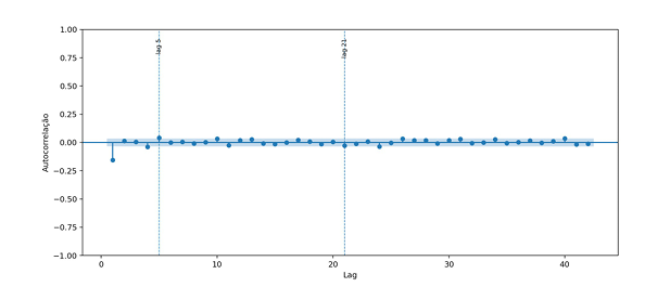
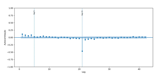
The ACF analysis of the out-of-sample errors indicated that, for RET_F1, most autocorrelations approached zero, but lag 1 was negative and the Ljung Box test remained significant (p-value of 2.04 * 10-13), suggesting very short-term residual dependence (Figure 7). For RISCO_F1, the residuals also rejected white noise (p-value of 7.31 * 10-165), with a negative peak at lag 21, which is more compatible with the construction of the risk measure than with economic seasonality (Figure 8).

Figure 7: Out-of-sample autocorrelation of RET_F1 residuals

Source: Original survey data

Figure 8: Out-of-sample autocorrelation of RISC_F1

Source: Original survey data

The comparison of training and testing metrics (Table 4) and the paired check on the test folds (Table 5) revealed distinct predictive performances for the targets. For RET_F1, LightGBM outperformed the reference model (persistence baseline) in training and testing, with MAE of 0.008081 and RMSE of 0.012398 on average across the folds. For RISCO_F1, the reference model was superior, with MAE of 0.000436 and RMSE of 0.001227. This indicates that the daily return may benefit from the combination of past information, while the very short-term risk is better described by the continuity of the series.

Table 4. Train and test metrics by model

Goal	Model	MAE training	RMSE train	MAE test	RMSE test
RET_F1	LightGBM	0.007830	0.012665	0.008081	0.012398
RET_F1	Persistence baseline	0.011477	0.018970	0.012130	0.018903
RISK_F1	Persistence baseline	0.000450	0.001251	0.000436	0.001227
RISK_F1	LightGBM	0.001144	0.002363	0.001732	0.003432

Source: Original survey data

Table 5. Paired comparison for RET_F1 and RISK_F1 in the test folds

Goal	Model	MAE	RMSE	Observation
RET_F1	LightGBM	0,008081	0,012888	3280
RET_F1	Persistence baseline	0,012130	0,019588	3280
RISK_F1	Persistence baseline	0,000436	0,001379	3280
RISK_F1	LightGBM	0,001732	0,004265	3280

Source: Original survey data

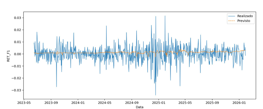
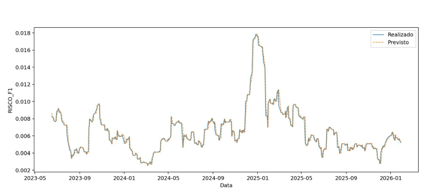
The comparison between observed and predicted values in the last test period (Figure 9) showed that LightGBM followed the local direction of RET_F1 oscillations better than the naive benchmark, despite deviations in abrupt changes. For RISCO_F1, persistence reproduced the current level of the series more closely, consistent with the observed continuity (Figure 10).

Figure 9: Observed and predicted values of RET_F1 in the last test

Source: Original survey data

Figure 10: Observed and predicted values of RISK_F1 in the last test

Source: Original survey data

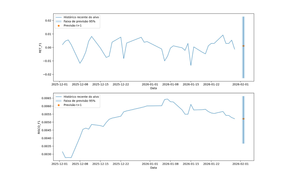
The final nowcast at t+1, based on the best validated model, was generated with information available on Jan. 30, 2026 for Feb. 02, 2026 (Table 7). For RET_F1, LightGBM predicted 0.001175, with a 95% empirical range between -0.022796 and 0.022847. For RISCO_F1, the persistence model predicted 0.005213, with a range between 0.003661 and 0.006626. The narrower band for risk reinforces its greater temporal continuity (Figure 11; Hyndman and Athanasopoulos, 2021).

Figure 11: t+1 return and risk Nowcast with 95% interval

Source: Original survey data

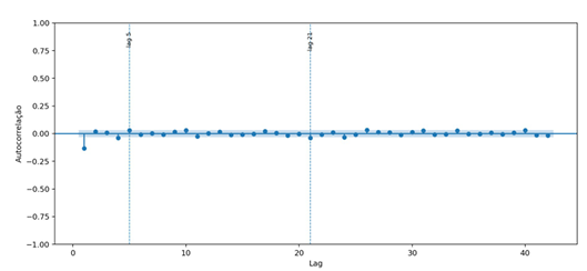
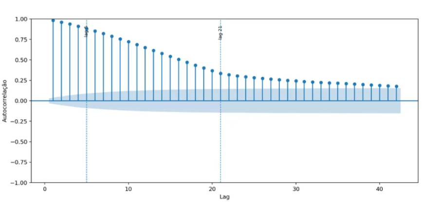
The re-presentation of the autocorrelation of the targets (Figure 12 for RET_F1 and Figure 13 for RISCO_F1) reinforced the structural difference between return and risk, with today’s risk carrying more information about tomorrow’s risk than today’s return about tomorrow’s return (Hyndman and Athanasopoulos, 2021; Ljung and Box, 1978).

Figure 12: Autocorrelation of return at t+1

Source: Original survey data

Figure 13: Autocorrelation of risk at t+1

Source: Original survey data

The fitted Hidden Markov Model (HMM) identified two persistent states in the sample, with high probabilities of remaining in the same state daily (p00 = 0.988733 and p11 = 0.973141), as per Table 6. This suggests the existence of distinct market contexts over time (Hamilton, 1989; Rabiner, 1989). However, the HMM was primarily used as a descriptive tool, given the limited coverage of ANBIMA’s term structure of interest rates (TSIR) data, which prevented its central incorporation into the predictive block.

Table 6. HMM in full sample

Measure	Result
State Counting	{“0”: 2782, “1”: 1164}
Final log-likelihood	-7327,915014
p00	0,988733
p01	0,011267
p10	0,026859
p11	0,973141

Source: Original survey data

Table 7. Final nowcast at t+1 with 95% empirical interval

Goal	database t	Forecast date t+1	Model	Point Forecast	Lower bound 95%	Upper limit 95%
RET_F1	2026-01-30	2026-02-02	LightGBM	0,001175	-0,022796	0,022847
RISK_F1	2026-01-30	2026-02-02	Persistence baseline	0,005213	0,003661	0,006626

Source: Original survey data

The results demonstrate a clear distinction between the daily return of the Tesouro IPCA+ and its risk. The return, which reacts to price revisions and unexpected shocks, allows for a moderate predictive gain with more flexible models like LightGBM. In contrast, the risk, built on a rolling window, exhibits strong temporal continuity, being better predicted by a simple persistence rule. The temporal heterogeneity of the sample, evidenced by the two regimes identified by the HMM, is relevant for economic interpretation, indicating that the market does not behave homogeneously over time. Although inflationary dynamics and risk persistence are important, the historical limitation of ANBIMA curves restricted the broader incorporation of the term structure of interest rates into the main predictive model.

In summary, the study indicated that the daily return of Tesouro IPCA+ exhibits low persistence and can be moderately predicted by machine learning models, while the very short-term risk demonstrates high persistence and is better estimated by repeating the most recent value. This distinction highlights the need for differentiated predictive approaches for each target, providing an objective basis for decisions in volatile market environments.

4. Conclusion

The study sought to estimate and evaluate nowcasting models for the return and risk of IPCA+ Treasury bonds, considering market arrangements and the influence of inflationary shocks, expectations, and regimes on prices and profitability. It was found that the daily return of the IPCA+ Treasury oscillated around zero, admitting a moderate predictive gain with the LightGBM model, which surpassed the persistence benchmark. In contrast, the risk at t+1 exhibited strong persistence, being better predicted by the simple repetition of the most recent value. This distinction highlighted the need for differentiated predictive approaches for each target. It was also observed that the temporal heterogeneity of the sample, evidenced by two regimes identified by a Hidden Markov Model, is relevant for economic interpretation, indicating that market behavior is not homogeneous over time.

The main contribution of this work lies in offering an objective basis for decisions in volatile market environments, by combining point forecast, out-of-sample validation, and empirical interval for the one-day horizon. The findings indicate that return and risk require distinct predictive treatments, providing valuable insights for investors and managers. However, the limited historical coverage of ANBIMA curves restricted the broader incorporation of the term structure of real interest rates, nominal rates, and implied inflation into the main predictive block. For future studies, it is suggested that consistent expansion of these curves may indicate whether regime segmentation adds economic content and additional predictive value, deepening the understanding of how inflationary shocks and market expectations affect the pricing of these securities.

Bibliographic References

Banco Central do Brasil [BACEN]. 2022. Relatório de Inflação. Disponível em: https://www.bcb.gov.br/content/ri/relatorioinflacao/202212/ri202212p.pdf. Acesso em: 02 abr. 2026.

Bańbura, M.; Giannone, D.; Reichlin, L. 2010. Nowcasting. ECB Working Paper Series – European Central Bank (175): 1-40.

Corsi, F. 2009. A Simple Approximate Long Memory Model of Realized Volatility. Journal of Financial Econometrics 7(2): 174-196.

Ferreira, R. G. 2015. Tesouro Direto e Outros Investimentos Financeiros: LTN, LFT, NTN, CDB, RDB, LCI e LI: Planos Financeiros e Atuariais de Aposentadoria. Atlas. São Paulo.

Hamilton, J. D. 1989. A New Approach to the Economic Analysis of Nonstationary Time Series and the Business Cycle. Econometrica 57(2): 357-384.

Hodson, T. O. 2022. Root Mean Square Error or Mean Absolute Error. When to Use Them or Not. Geoscientific Model Development 15(14): 5481-5487.

Hyndman, R. J.; Athanasopoulos, G. 2021. Forecasting: Principles and Practice. 3 ed. OTexts. Melbourne. Disponível em: https://otexts.com/fpp3/. Acesso em: 02 abr. 2026.

Júnior, J. B. A.; Tavares, L. A. P. 2024. Rentabilidade dos títulos do tesouro. Uma análise de séries temporais e janelas móveis. Revista Processus de Estudos de Gestão, Jurídicos e Financeiros 15(48): 1-19.

Ke, G.; Meng, Q.; Finley, T.; Wang, T.; Chen, W.; Ma, W.; Ye, Q.; Liu, T.-Y. 2017. LightGBM. A Highly Efficient Gradient Boosting Decision Tree. Advances in Neural Information Processing Systems 30: 3146-3154.

Ljung, G. M.; Box, G. E. P. 1978. On a Measure of Lack of Fit in Time Series Models. Biometrika 65(2): 297-303.

Minella, A.; Freitas, P. S.; Goldfajn, I.; Kfoury, M. M. 2003. Inflation Targeting in Brazil: Constructing Credibility under Exchange Rate Volatility. Journal of International Money and Finance 22(7): 1015-1040.

Ministério da Fazenda [GOV]. 2025. Investimentos no Tesouro Direto somam R$ 7,26 bilhões em julho, aponta Tesouro Nacional. Disponível em: https://www.gov.br/fazenda/pt-br/assuntos/noticias/2025/agosto/investimentos-no-tesouro-direto-somam-r-7-26-bilhoes-em-julho-aponta-tesouro-nacional. Acesso em: 02 abr. 2026.

National Institute of Standards and Technology [NIST]. 2026. Normal Probability Plot. Disponível em: https://www.itl.nist.gov/div898/handbook/eda/section3/normprpl.htm. Acesso em: 02 abr. 2026.

Perlin, M. 2016. A Microestrutura do Tesouro Direto: Sazonalidade do Fluxo de Ordens e o Processo de Formação de Spreads. Economia Aplicada 20(3): 253-272.

Portal do Investidor [GOV]. 2022. Tesouro IPCA+. Disponível em: https://www.gov.br/investidor/pt-br/investir/tipos-de-investimentos/titulos-publicos/tesouro-ipca. Acesso em: 02 abr. 2026.

Rabiner, L. R. 1989. A Tutorial on Hidden Markov Models and Selected Applications in Speech Recognition. Proceedings of the IEEE 77(2): 257-286.

Silva, C. G.; Leme, M. C. S. 2008. Inflation and Interest Rate. Which One Is More Persistent in Brazil? Anais do XXXVI Encontro Nacional de Economia.

Tesouro Nacional [GOV]. 2025. Tesouro Direto bate recordes de vendas, número de operações, resgates e vendas líquidas em dezembro. Disponível em: https://www.gov.br/tesouronacional/pt-br/noticias/investimentos-no-tesouro-direto-somam-r-8-55-bilhoes-em-dezembro-maior-valor-da-serie-historica. Acesso em: 02 abr. 2026.

Tesouro Transparente. 2026. Taxas dos Títulos Ofertados pelo Tesouro Direto. Disponível em: https://www.tesourotransparente.gov.br/ckan/dataset/taxas-dos-titulos-ofertados-pelo-tesouro-direto. Acesso em: 02 abr. 2026.

Article originating from the Course Conclusion Work of the Specialization in Data Science and Analytics of the MBA USP/Esalq

To learn more about the course, click here and access the MBX Academy platform

Most recent

Economy, Investments And Banking

October 23, 2026

Financial Education, Behaviors and Biases in Financial Decision Making

October 22, 2026

Challenges and Possibilities of the First School Year of Children with ASD for Teaching Work

October 22, 2026

Consumer Journey in the Decision to Purchase Infoproducts in the Digital Environment

October 22, 2026

Psychosocial Risks and Mental Health at Work in a Banking Institution

October 22, 2026

Digital Observatory of the Amazon: Data Science Applied to the Analysis of Social, Economic, Environmental, and Health Indicators

October 22, 2026

Continuous Learning as a Factor of Organizational Growth in the Perception of Collaborators

October 22, 2026

Statistical Regression in Microgrids for Operational Performance Estimation: Campusgrid Case

October 22, 2026

Forecast of Aggregate Default in the Brazilian Financial System by Sarimax Model with Macroeconomic Variables

October 22, 2026

Stakeholder Engagement Factors in International Technology Transfer to a Public Hospital

Personal financial management represents a growing challenge, influenced by cognitive biases that affect decision-making, even in individuals with high knowledge. The present study analyzed the relationship between the level of financial education and the occurrence of behavioral biases in the financial decision-making of adults residing in Brazil. An applied, quantitative, and descriptive-correlational field survey was conducted by administering a structured questionnaire to 163 respondents. The instrument included sociodemographic variables, financial knowledge and habits, and hypothetical situations to identify cognitive biases. The results indicated that higher levels of financial education were associated with better financial control, saving, and investment practices, with significant correlations with income and schooling. However, the presence of behavioral biases (anchoring, loss aversion, scarcity, optimism/negativity, present bias, status quo, overconfidence, and mental accounting) persisted even among individuals with higher schooling and income, with no statistically significant association with the analyzed sociodemographic variables. It was concluded that financial education, although essential for financial organization and control, was not sufficient to neutralize the influence of cognitive biases. The incorporation of behavioral approaches into financial education programs is suggested.

Keywords: Financial behavior; Behavioral economics; Personal finance; Cognitive heuristics; Cognitive biases.

October 22, 2026

Challenges and Possibilities of the First School Year of Children with ASD for Teaching Work

The inclusion of children with Autism Spectrum Disorder (ASD) in Early Childhood Education presents significant challenges, given the difficulty of adapting to new environments and the intensity of stimuli. The objective was to analyze the teaching performance in Early Childhood Education in the initial schooling process of children with ASD. A case study was conducted, using narrative interview as a data production technique. The results revealed that the teaching performance was characterized by mediation and affection practices, with the flexibility of routine and the use of playful resources as essential strategies for the child’s development and sensory organization. The importance of the school support professional for the success of the pedagogical work was also highlighted. The child’s integral development was promoted through intentional teaching actions that prioritized environmental adaptation, strengthening of bonds, and attention to the specific needs of ASD. As a contribution, a guide of pedagogical strategies aimed at welcoming children with ASD in public daycare centers was developed.

Keywords: Early Childhood Education; School Inclusion; Teacher Narratives; Inclusive Pedagogical Practices; Autism Spectrum Disorder.

October 22, 2026

Consumer Journey in the Decision to Purchase Infoproducts in the Digital Environment

The expansion of e-commerce and technological transformation have driven the need to understand consumer behavior regarding infoproducts, whose perceived experience has become crucial for professional development. The study aimed to analyze the factors that influenced the purchase decision of infoproducts in the digital environment, considering the stages of the consumer journey. An applied, quantitative, and descriptive research was conducted through a field survey with 100 consumers from Serra Gaúcha. Data collection occurred via a structured questionnaire, using non-probabilistic sampling. The results revealed a qualified audience with strong “mobile-first” behavior. It was found that the availability of detailed information and social approval were the main attraction triggers in the pre-purchase phase. In the transactional and subsequent stages, the minimization of operational friction, the agility of immediate access, and system security proved crucial for conversion and satisfaction, although gaps in human support efficiency were identified. Retention was based on the trust generated by positive past experiences, overcoming the price factor. It was concluded that the infoproduct consumer journey operates as an integrated system, requiring alignment between technological infrastructure, content curation, and support humanization to ensure engagement.

Keywords: E-commerce; Consumer behavior; Consumer experience; Loyalty; Virtual business.

October 22, 2026

Psychosocial Risks and Mental Health at Work in a Banking Institution

Mental health in the workplace is a topic of growing relevance, impacting professional development and employee well-being. A study was conducted to identify aspects and situations that can influence absenteeism levels in a banking institution. The research involved 108 participants and used a structured questionnaire, based on the short version of COPSOQ II by Gonçalves (2021), which contained 45 closed Likert scale questions and two open-ended questions. Data were collected via an online platform and analyzed with a descriptive and quantitative approach. The results revealed a scenario that indicated the need for adjustments in the distribution of activities and in managers’ perception of behaviors and signs of disorders. Important evidence was identified in the participants’ open-ended responses. It was concluded that the study contributed to promoting the perception of a safe environment for mental health in the organization.

Keywords: Absences due to disorders; Professional development; Operational leadership; Medical leave; Mental health.

October 22, 2026

Digital Observatory of the Amazon: Data Science Applied to the Analysis of Social, Economic, Environmental, and Health Indicators

The state of Amazonas faced historical challenges in consolidating the Unified Health System (SUS), stemming from geographical barriers, socioeconomic inequalities, and structural limitations. This study described the development and implementation of a health information geoportal, designed to support monitoring, evaluation, and planning in the Amazonian context. A descriptive case study approach was adopted, based on documentary analysis and secondary data, covering the mapping of functionalities, technical infrastructure, and validation steps of the tool. The Portal was developed with open technologies and integrated multiple national databases, offering interactive dashboards, thematic maps, and a digital document repository. Among the results, highlighted were the georeferenced visualization of key indicators, the possibility of temporal comparative analyses, and the use of the platform in reviewing health plans and redirecting strategic actions. The portal can represent an advance in digital governance and evidence-based management, with potential for replication in other highly complex territories, provided it is accompanied by investments in technological infrastructure, professional training, and inter-institutional coordination.

Keywords: Amazon; Health Evaluation; Digital Health; Health Information Systems.

October 22, 2026

Continuous Learning as a Factor of Organizational Growth in the Perception of Collaborators

The impact of continuous learning and knowledge management on organizational growth was studied in a context of globalization and constant changes. The study’s objective was to analyze employees’ perception of learning culture and its importance for personal and professional development. Data were obtained through an anonymous survey, with a quantitative approach, using a form with “survey” type questions applied to 87 professionals from the technology, health, education, commerce, and services sectors. The results indicated that employees had a positive perception of the contribution of continuous learning to personal and organizational growth, recognizing its benefits for the development of new skills, innovation, and competitiveness. However, it was observed that the incentive for internal knowledge exchange and the offering of practical training still presented moderate levels of agreement. It was concluded that continuous learning significantly contributes to individual and organizational development, suggesting that companies should develop strategic policies for learning focused on new skills, aiming for greater competitive advantage and innovation.

Keywords: Continuous learning; Self-development; Organizational growth; Knowledge Management; Innovation.

October 22, 2026

Statistical Regression in Microgrids for Operational Performance Estimation: Campusgrid Case

A multiple statistical regression model was proposed to estimate the operational performance of UNICAMP’s CampusGrid microgrid, based on internal electrical quantities. The microgrid integrates photovoltaic generation, batteries, and a gas generator. Energy management system data were collected at five-minute intervals over one month. The Operational Reliability Index, defined as the ratio between supplied and demanded energy, was established as the dependent variable. The model was adjusted for the islanded operation mode, evaluating the impact of demand, state of charge, solar generation, and supplied energy. The results revealed high explanatory power, indicating that operational reliability depends on the interaction between supply and demand. It was observed that the nighttime period concentrated the highest rate of partial supply, attributed to the reduction in solar generation. It was concluded that multiple regression offers an interpretable and useful framework for microgrid monitoring and control strategy support.

Keywords: Battery storage; Photovoltaic generation; Reliability Index; Islanded operation; Energy Management System.

October 22, 2026

Forecast of Aggregate Default in the Brazilian Financial System by Sarimax Model with Macroeconomic Variables

Aggregate non-payment in the Brazilian financial system is a crucial indicator of credit risk, the prediction of which is regulated by CMN Resolutions n.° 4.557/2017 and 4.966/2021 for the prospective measurement of expected losses. Aggregate non-payment was modeled and predicted using the SARIMAX model, projecting its trajectory until December 2026 under optimistic, base, and pessimistic scenarios. 164 monthly observations (July/2012 to February/2026) and macroeconomic variables such as unemployment, Selic, IPCA, IBC-Br, and household debt were used. The specification with contemporaneous variables was selected based on information criteria and coefficient stability, and residual diagnostics confirmed statistical adequacy, with a MAPE of 3.12%. Historical non-payment ranged between 4.33% and 7.64%. The estimation identified unemployment (β = 0.2534; p < 0.001) and Selic (β = 0.2128; p < 0.001) as the main positive determinants, with strong temporal persistence (AR(1) = 0.8965). Selic showed increasing correlation with non-payment (r = 0.62 at lag 12), while unemployment demonstrated a contemporaneous effect (r = 0.33). Projections indicated non-payment between 6.30% and 7.98% in December 2026, with a range of 1.68 percentage points, highlighting direct implications for provisioning in financial institutions.

Keywords: Unemployment; Predictive modeling; Monetary policy; Loss provisioning; Time series.

October 22, 2026

Stakeholder Engagement Factors in International Technology Transfer to a Public Hospital

This study described the critical factors perceived for stakeholder engagement in international technology transfer in a public hospital, with a focus on planning. The objective was to describe these conditioning factors, according to the perception of professionals. A single case study was conducted, applying a questionnaire to 25 professionals and using content analysis, complemented by descriptive tabulations. The main obstacles identified were resistance to change (72%), funding (64%), lack of communication (60%), and bureaucracy (40%). Only 28% of respondents recognized the existence of adequate tools for stakeholder management, while 48% denied it and 24% did not know. Exploratory cross-tabulations indicated variations in the assessment of influence according to time of practice, but did not establish causal relationships. Lack of engagement was associated with delays, low adherence, waste of resources, communication failures, compromised knowledge absorption, and risks to patient safety. The conclusions were limited to the perceptions of the researched group and supported preliminary recommendations for intersectoral communication and coordination.

Keywords: Case study; Project Management; Health innovation; Stakeholders; Public sector.

Economy

October 19, 2026

End of the 6×1 scale: what do the numbers allow us to conclude?

Following the promulgation of the end of the 6×1 shift system, the debate on the shorter workday moves to implementation and requires distinguishing social benefits from economic costs. The end of the 6×1 shift system transitioned from legislative discussion to a constitutional change in Brazil. On October 16, 2026, the National Congress promulgated Constitutional Amendment No. 141/2026, originating from Proposal […]

Artificial Intelligence

October 16, 2026

Why study if AI exists?

When answers become easy, learning comes to mean more than just arriving at them. Why do I need to learn this if I can ask an artificial intelligence? This type of question has accompanied education for decades. Why learn an operation if a calculator exists? Why memorize information if it can be found […]

Tax Management

October 15, 2026

Pink tax and the gender of price

How different marketing treatments for men and women are incorporated by consumption taxation Imagine a shelf on which two razors of the same brand and intended for the same purpose are displayed side by side: one has dark packaging and promises strength, precision, and efficiency; the other comes in shades of pink or […]

Health

October 13, 2026

The missing link in health transformation

Why is innovation not enough to drive changes in organizations and health systems Digital transformation has become a strategic priority for health systems worldwide. Electronic health records, artificial intelligence, telemedicine, remote monitoring, and data analysis are now part of the strategic agenda of governments and health organizations. Paradoxically, […]

Marketing

October 09, 2026

Bitcoin or pets: what Artificial Intelligence would not see

A real-life consumer intelligence case shows what gets left out of the brief A few years ago, an American insurance company hired a specialized consumer intelligence firm to answer three questions: The insurer was also considering launching paid insurance in bitcoin. At the time, the consultancy’s workflow was as follows: the analyst created a query […]

School Management

October 06, 2026

The school is not a casino: when trading cards become currency in the playground

Why, for certain students, does school manage to offer so few experiences of achievement? The World Cup is over. Brazil left the competition, the school holidays came, the final was played and the football calendar moved on. It would be reasonable to imagine that, with the end of the tournament and the return to classes, […] would also begin

Energy Transition

September 30, 2026

Renewable energies: the Brazilian advantage

Brazil needs to invest in the capacity to transform natural resources into innovation, productivity, and development. Talking about energy is talking about development. Behind industry, transportation, services, cities, and increasingly artificial intelligence, there is an energy infrastructure that sustains the economy. Understanding a country’s energy matrix is understanding […]

Data Analysis

September 30, 2026

When the data changes, has reality changed?

An analysis of almost 20 million teaching positions-year between 2020 and 2025 shows how changes in population composition and record production can alter the interpretation of historical series Between 2020 and 2025, the number of formal teaching employment positions identified in RAIS (Annual Relation of Social Information), from the Ministry of Labor, […]

Artificial Intelligence

September 28, 2026

Artificial intelligence and the trends

Why do so many people join in on the fun with ChatGPT? I was never the trend person. I still am not. Some pass through my timeline, I see them, I find them interesting but not to the point of trying them out. This was the case, inclusive, with some recent waves of images made by artificial intelligence, like the 80s trend, the one that […]

Tax Management

September 01, 2026

Tax reform and estate planning in the countryside

Efficiency in managing taxes facilitates governance and allows for the organization of family succession. Rural wealth organization has become a strategic measure in light of the tax reform in Brazil, which came into effect this year. The planning of activities and rural wealth management, through tools such as the transition from an Individual to […]

Renata de Gaspari Valdejão Almeida

Artificial Intelligence

August 05, 2026

Inside the company and off the radar: the risks of Shadow AI

According to Microsoft, 75% of professionals already use artificial intelligence at work without company approval. The use of generative artificial intelligence is already part of the corporate routine. Tools like ChatGPT, Copilot, and other platforms help professionals produce texts, analyze data, create presentations, and accelerate tasks in practically all sectors. But this advance […]

Renata de Gaspari Valdejão Almeida

Strategy

July 02, 2026

The future as a competence

Academic interest reinforces the projection of scenarios as an essential tool for decision-making. While some companies are still trying to get the next step right, others are already working with multiple possible futures — and preparing for all of them. But after all, what does it mean to “think about the future”? Is it a trend, a strategy, or a new competence that […]

Renata de Gaspari Valdejão Almeida

Innovation

Technology

May 21, 2026

Agro SP Corridor: innovation, institutional articulation and future

Pecege commands the executive operation of the 400 km ecosystem activities that became known as the Brazilian agro Silicon Valley In 2025, in addition to taking over the management of the Piracicaba Technology Park, the Pecege Institute was also designated to command the executive operation of the State Agribusiness Innovation Corridor activities, the so-called […]

Education

April 27, 2026

How to turn a TCC into a business

New management of the Piracicaba Technology Park offers consulting to MBA graduates The new project director of the Piracicaba Technology Park (PTP), Alexandre Barreto, often says that one of the greatest rewards he has ever had in life was seeing his MBA USP/Esalq students structure companies from their final projects […]

Technology

March 20, 2026

The human repertoire in the age of AI

Critical thinking and creativity are irreplaceable in the work of a marketing professional Artificial Intelligence (AI) is capable of incredible feats, but it does not yet possess the judgment, empathy, intuition, and strategic creativity necessary to do the job of a good marketing professional. In this area, it is important to know how to use the tool to automate […]

Renata de Gaspari Valdejão Almeida

Agribusiness

Innovation

February 23, 2026

ESG as a growth strategy in a cooperative in RS

Santa Clara balances social and environmental responsibility with innovation Founded in 1911 by Italian immigrants in Carlos Barbosa, in the Serra Gaúcha region, Cooperativa Santa Clara is an example that it is possible to balance economic growth with social and environmental responsibility. From a small cheese production company, the organization has evolved into a […]

Renata de Gaspari Valdejão Almeida

Agribusiness

Innovation

January 22, 2026

Brazil free of Foot-and-Mouth Disease: what changes for Brazilian beef?

With a herd of over 200 million head of cattle, the country is currently the leader in exports. Brazil recently received, for the first time, the certification of country free of foot -and-mouth disease without vaccination, conferred by the World Organisation for Animal Health (WOAH). The seal strengthens the country’s position as a reliable supplier of meat for the […]

Renata de Gaspari Valdejão Almeida

Innovation

December 09, 2025

Innovation: the new cycle of the Piracicaba Technology Park

Instituto Pecege assumes management, betting on the creation of new businesses Starting in 2026, Instituto Pecege will assume the management of the Piracicaba Technology Park (PTP). Among its responsibilities will be the administration, operation, maintenance, and expansion of the park, in addition to fostering activities in innovation, entrepreneurship, and science and technology. The choice was made […]

Renata de Gaspari Valdejão Almeida

July 06, 2026

Large-Scale Architecture: DSR-SCRUM Change Management

Mônica Alessandra Guerios; Maria do Carmo Assis Todorov Abstract generated by ResumeAI, an artificial intelligence solution developed by Instituto Pecege focused on synthesis and writing. Architecture and urbanism are configured as essential bases in an increasingly complex and challenging urban space, where the intrinsic connection between social, environmental, and technological issues […]