
September 10, 2026
Multilevel Modeling in the Estimation of Sugarcane (Saccharum Spp.) Productivity in Production Units in the Southeast Region of Mato Grosso do Sul
Ferdinando Yoshio Agapito Urasaki; Luiz Gustavo Antônio de Souza
DOI: 10.22167/2675-6528-202602215
Article derived from a Final Course Work (TCC), with content based on the student’s original work and adapted to the editorial format of the Revista E&S with the support of the ResumeAI tool, an artificial intelligence solution developed by the Pecege Institute for textual synthesis and organization.
Summary
The productivity estimation is essential for agricultural planning, but the clustering structure of agronomic data frequently violates the independence assumption of classical regression models. The accuracy of multilevel models with cross-classification was evaluated in predicting the agricultural yield of sugarcane in the southeastern region of Mato Grosso do Sul, covering the harvests from 2019/2020 to 2023/2024. The study analyzed 29,674 observations, organized across 10,336 plots and 30 varieties. Biophysical and agrometeorological predictors were integrated, applying the “Step-Up” strategy for constructing the multilevel structure and variance decomposition. The results showed that the approach adequately partitioned the spatial, genetic, and temporal variance, successfully quantifying the genotype-environment interaction. The final adjustment with random slopes (M7) explained 81.1% of the total variance and achieved a Root Mean Square Error (RMSE) of 10.24 t ha⁻¹. The 9.8% difference measured between the marginal and conditional Pseudo-R² demonstrated the relevant explanatory gain generated by cross-classification. The predictive performance was comparable to the accuracy reported by Machine Learning algorithms, maintaining the parametric rigor and interpretability of agronomic predictors. It was concluded that multilevel modeling constituted a robust and transparent analytical tool for productivity estimation and planning in the sugarcane sector.
Keywords: Agrometeorology; Sugarcane; Cross-classification; Multilevel modeling; Agricultural yield.
1. Introduction
Sugarcane (Saccharum spp.) stands out as one of Brazil’s main agricultural commodities, alongside soybeans and corn. Together, these crops occupy approximately 6.9% of the national territory and over 70% of the cultivated agricultural area (EPE, 2024b). In addition to sugar production, the crop is fundamental for generating ethanol and for utilizing byproducts, such as vinasse in fertigation and bagasse in the cogeneration of electrical energy (Avilez et al., 2018; EPE, 2024b). This utilization is reflected in the Brazilian energy matrix, where sugarcane biomass and its derivatives represent 16.8% of the domestic supply, being the second largest energy resource in the country, surpassed only by petroleum (EPE, 2024a).
In this context, the southeastern region of Mato Grosso do Sul is configured as a strategic hub for sugarcane production, driven by its high bioenergetic density (BIOSUL, 2024) and favorable edaphoclimatic conditions (Manzatto et al., 2009). To ensure the operational efficiency of production units, accuracy in productivity estimation, measured in tons of sugarcane per hectare (TCH), is crucial. Such precision is decisive for harvest planning and logistical optimization, ensuring continuous supply to the industrial plant (Silva A.S. et al., 2022).
The productive potential of sugarcane can reach 400 t ha⁻¹ per year, due to its high photosynthetic efficiency. However, yield is conditioned by a complex interaction of environmental and operational factors, notably water and nutritional availability (Silva et al., 2012). As a semi-perennial crop, with an average cycle of five harvests, sugarcane presents four distinct phenological phases (sprouting, tillering, vegetative growth, and maturation), each with specific water demands. The initial phases are particularly sensitive to water stress, and vegetative growth is the most critical period, while moderate water restriction during maturation favors sucrose accumulation (Avilez et al., 2018). The total water demand varies between 1,500 and 2,500 mm, and the optimal temperature is between 25 and 33 °C (Almeida et al., 2008). Extreme events, such as frosts, can also significantly compromise production, with severity proportional to the intensity and duration of the phenomenon (Fiorentin et al., 2016).
With the objective of quantifying the impact of these agrometeorological factors and enabling crop prediction, sugarcane productivity modeling has been widely explored. Methods such as multiple linear regression have been used to estimate annual productivity based on variables like irrigation, precipitation, and air temperature (Silva A.S. et al., 2022), or to correlate biomass production with vegetation indices (Silva M.G.S. et al., 2022). Scarpari (2002) also proposed the prediction of agricultural productivity by integrating precipitation and growing degree day data.
Despite the advances represented by these models, multiple linear regression often violates the assumption of independence of observations, which can lead to incorrect error estimates and optimistic confidence intervals (Gelman and Hill, 2006). In the agricultural context, productivity is not an isolated event, but the result of complex structural interdependencies. For example, climatic variations in one harvest affect multiple areas simultaneously, the variety establishes common biological potentials among plots, and the succession of cycles in the same plot induces temporal autocorrelation.
To adequately address these interdependencies, multilevel modeling emerges as a more robust analytical alternative compared to classical regression. In agricultural data, the organization of observations rarely follows a strict hierarchical structure, as grouping factors such as variety and crop often intersect over time across plots, configuring a cross-classification structure. This approach allows for the isolation of variance intrinsic to each context (spatial, genetic, and temporal), correcting the underestimation of standard errors, a common problem in models that ignore this complexity (Gelman and Hill, 2006). Thus, this study is justified by the need for an analytical tool that not only predicts productivity with accuracy but also preserves the parametric rigor and interpretability of agronomic predictors.
Under this premise, the objective was to evaluate the accuracy of multilevel models with cross-classification in predicting sugarcane productivity in production units in the southeastern region of Mato Grosso do Sul, covering the historical series of harvests from 2019/2020 to 2023/2024. Specifically, we sought to decompose the total variance to quantify the influence of the plot, variety, and harvest components in explaining productive variability, as well as to determine the relative contribution of biophysical and agrometeorological predictors on the TCH variance.
2. Material and Methods
The study was conducted in the southeastern region of Mato Grosso do Sul, encompassing the municipalities of Angélica, Deodápolis, Glória de Dourados, Ivinhema, Jateí, Naviraí, Nova Andradina, and Novo Horizonte do Sul. The choice of this region was justified by its strategic relevance and the robustness of historical agronomic data series, which are fundamental for adjusting productivity prediction models at the local level.
The database was structured from the integration of operational records, multispectral remote sensing data, and exogenous environmental variables, categorized as:
- Agronomic: Records of sugarcane production units, including soil characterization, planting and harvesting dates, genetic material (variety), cutting number, agricultural productivity (TCH), and plot geometry.
- Environmental and Spectral Variables:
- Remote Sensing: Sentinel-2 (MSI) satellite imagery, processed at Level 2A, with spatial resolution of 10 m and 20 m and a five-day revisit, for the extraction of 11 spectral indices.
- Precipitation: Estimates from the Climate Hazards Group InfraRed Precipitation with Station data (CHIRPS) collection, with daily temporal resolution and 0.05° (~5.5 km) spatial resolution.
- Topography: Digital Elevation Model (DEM) derived from the Shuttle Radar Topography Mission (SRTM), with a spatial resolution of 1 arc-second (~30 m).
- Meteorology: Reanalysis data from the ERA5-Land collection, with spatial resolution of 0.1° (~11 km) and daily temporal resolution, for extracting air temperature (minimum, average, and maximum), dew point temperature, vector components of wind, and shortwave solar radiation.
The workflow was outlined in eleven steps: (i) cleaning and engineering of agronomic attributes; (ii) geometric processing for zonal statistics; (iii) monthly collection of spectral indices; (iv) monthly collection of agrometeorological variables; (v) structuring of spectral and agrometeorological time series; (vi) treatment of gaps in spectral indices; (vii) synchronization of cycles and adjustment of management dates; (viii) consolidation of metrics and temporal integration; (ix) variable selection and dimensionality reduction; (x) specification of the multilevel model; and (xi) validation and performance evaluation of the models.
All processing was implemented in Python language (version 3.12), using the Pandas, GeoPandas, and NumPy libraries. The integration and cloud processing of spectral indices and agrometeorological variables were operationalized via the Google Earth Engine API (ee library) and Geemap. For multilevel modeling, the Pymer4 library was used, which provides an interface with the lme4 package algorithms of the R language.
The treatment of raw agronomic data (225,992 records) began with the removal of observations with missing data on productivity, cutting number, and production environment, restricting the sampling to own production and partnership modalities. Temporal consistency and area parity were ensured by removing plots with multivariate plantings. The analytical scope covered the crop seasons 2019/2020 to 2023/2024, from the first to the seventh cut, and the 30 most representative varieties. Productivity outliers were identified by the Interquartile Range (IQR) method, with a multiplier of 1.5, stratified by cutting number and production environment. Consistency between alphanumeric and vector attributes was validated, discarding records with an absolute divergence greater than 0.025 ha. The resulting database totaled 32,033 records.
For the refinement of the sampling, plots with an area greater than 1.0 ha were selected. The original geometries were redefined by a spatial retraction of 20 m to mitigate the edge effect, ensuring that only internal pixels were processed. The resulting 30,953 records served as a vector base for zonal statistics on the Google Earth Engine (GEE) platform.
For the monthly collection of spectral indices, Sentinel-2 images with less than 20% cloud cover were pre-selected, applying a boolean filter based on the scene classification layer (SCL) generated by the Sen2Cor algorithm. The data were organized into monthly compositions, using the median of each pixel to eliminate atmospheric noise. 11 spectral indices derived from different bands were calculated, as detailed in Table 1.
Table 1. Relation of spectral indices and respective formulations.
| Index | Acronym | Equation | Reference |
|---|---|---|---|
| normalized difference vegetation index | NDVI | (PNIR – PR) / (PNIR + PR) | Rouse et al. (1974) |
| normalized difference green vegetation index | GNDVI | (PNIR – PG) / (PNIR + PG) | Gitelson et al. (1996) |
| soil-adjusted vegetation index | SAVI | (PNIR – PR / (PNIR + PR + L)) * (1 + L) | Huete (1988) |
| modified soil adjusted vegetation index 2 | MSAVI2 | (2PNIR + 1 – sqrt((2PNIR + 1)^2 – 8(PNIR – PR))) / 2 | Qi et al. (1994) |
| highlighted vegetation index | EVI | 2.5 * (PNIR – PR / (PNIR + 6PR – 7.5PB + 1)) | Huete et al. (2002) |
| normalized difference water index | NDWI | (PNIR – PSWIR1) / (PNIR + PSWIR1) | Gao (1996) |
| edge index of red by normalized difference | NDRE | (PRE2 – PRE1) / (PRE2 + PRE1) | Barnes et al. (2000) |
| red edge chlorophyll index | CIre | (PRE3 – 1) / PRE1 | Gitelson et al. (2005) |
| inverted red-edge chlorophyll index | IRECI | (PRE3 – PR) / (PRE1/PRE2) | Frampton et al. (2013) |
| leaf area index of sentinel-2 | SeLI | (PNIR – PRE1) / (PNIR + PRE1) | Pasqualotto et al. (2019) |
| wide dynamic range vegetation index | WDRVI | (PNIR – PR) / (aPNIR + PR) | Gitelson (2004) |
Source: Original survey data. Note: α = 0.1; L = 0.5. Sentinel-2 bands: B2 (B), B3 (G), B4 (R), B5 (RE1), B6 (RE2), B7 (RE3), B8 (NIR), B11 (SWIR1).
The monthly collection of agrometeorological variables used reanalysis data and satellite estimates (CHIRPS and ERA5-Land) to ensure temporal continuity and spatial coverage. Indicators were structured into five axes: water supply (precipitation – P), thermal regime (minimum, average, and maximum temperatures – Tmin, Tmed, Tmax), energy availability (incident shortwave solar radiation – Rs), evaporative demand (reference evapotranspiration – ET0), and atmospheric stress (vapor pressure deficit – VPD). Thermal accumulation was quantified by daily degree-days (GDD) with a Tbase of 18 °C and a cutoff temperature (Tcut) of 35 °C. ET0 was estimated by the Penman-Monteith method. After daily computation, the matrix time series were aggregated into monthly compositions, using the sum reducer for flux variables (P, ET0, GDD, and Rs) and the average for state variables (Tmin, Tmed, Tmax, and VPD). The set of indicators and aggregation methods is presented in Table 2.
Table 2. Agrometeorological indicators and aggregation methods.
| Indicator | Acronym | Unit | Representation | Aggregation | Reference |
|---|---|---|---|---|---|
| precipitation | P | mm | pluvial water supply | sum | CHIRPS |
| minimum temperature | Tmin | °C | lower thermal limit | average | ERA5-Land |
| average temperature | Tmed | °C | average thermal state | average | ERA5-Land |
| maximum temperature | Tmax | °C | upper thermal limit | average | ERA5-Land |
| shortwave solar radiation | Rs | MJ · m⁻² | solar energy supply | sum | ERA5-Land |
| reference evapotranspiration | ET₀ | mm | potential water demand | sum | Allen et al. (1998) |
| accumulated degree-days | GDA | °C | phenological thermal accumulation | sum | Villa Nova et al. (1972) |
| vapor pressure deficit | VPD | kPa | hygrometric stress | average | ERA5-Land |
Source: Original survey data.
For the systematization of time series, the monthly matrix data of spectral index collections and agrometeorological variables were integrated into the geometries of the plots via zonal statistics on the GEE platform. The average values in the plot were computed with an arithmetic reducer, with an output spatial scale of 20 m, converting the matrix data into tabular attributes.
The internal gaps of the spectral indices were treated via linear interpolation. For the ends of the series, where interpolation was not feasible, persistence imputation (“forward fill” and “backward fill”) was applied, propagating the last valid observed value. The series were extended with a temporal window of 100 days before and after the limits of each cycle to prevent mathematical distortions.
The time series of spectral indices were smoothed with the Savitzky-Golay polynomial filter (second-order polynomial, five-observation moving window). Cycle boundaries were adjusted based on the spectral response of the smoothed NDVI, using local minima detection within a 90-day tolerance window around the recorded operational dates.
With the cycle limits adjusted, the monthly time series were aggregated into fixed chronological windows: F1 (30 to 120 days after the cycle start) and F2 (120 to 270 days). For the 11 spectral indices, the temporal integral (AUC) was calculated using the trapezoidal rule. The agrometeorological flux variables (P, ET0, GDD, and Rs) were integrated by summation, and the state variables (Tmin, Tmed, Tmax, and VPD) by arithmetic mean. Each attribute was identified by a specific nomenclature. This approach resulted in a set of 38 biophysical and agrometeorological characteristics across 29,674 observations.
For the selection of variables and dimensionality reduction, the Maximum Relevance and Minimum Redundancy (mRMR) method was used, which prioritizes variables with greater statistical dependence on the target variable and lower redundancy. After ranking, the 10 most relevant variables were selected. Subsequently, to mitigate multicollinearity, diagnosis was performed via Variance Inflation Factor (VIF), iteratively excluding variables with VIF greater than five, resulting in a set of six variables. The quantitative variables were centered on the grand mean.
The construction of the multilevel model adopted the “Step-Up” strategy, which consists of adding increasing parametric complexity. The statistical procedure began with the estimation of unconditional models to partition the total variance of productivity (TCH) associated with the spatial (plot), genetic (variety), and temporal (crop) contexts.
The M0 model established the baseline of the variance, including only the random intercept for the plot:
Y_i = beta_0 + u_t[i] + e_i (1)
Where: Y_i: productivity (TCH) in observation i; beta_0: global fixed intercept; u_t[i]: random plot effect; e_i: residual error.
The M1 and M2 models independently tested the inclusion of variance components associated with variety and crop, respectively:
M1: Random Intercept for Lot and Variety
Y_i = beta_0 + u_t[i] + v_v[i] + e_i (2)
Where: v_v[i]: random effect of the variety.
M2: Random Intercept for Lot and Harvest
Y_i = beta_0 + u_t[i] + w_s[i] + e_i (3)
Where: w_s[i]: random effect of the crop.
In the M3 model, random intercepts for plot, variety, and crop were incorporated simultaneously, consolidating the cross-classification structure:
M3: Cross-validation
Y_i = beta_0 + u_t[i] + v_v[i] + w_s[i] + e_i (4)
The estimation of variance components and parameters was performed using the Restricted Maximum Likelihood (REML) method. To evaluate the statistical fit gain, the Bayesian Information Criterion (BIC) and the Likelihood Ratio Test (LRT) were used, with adjustments by Maximum Likelihood (ML) for comparing models with different fixed effects structures.
With the variance components consolidated in M3, the categorical fixed-effect variables were added. Model M4 incorporated the cutoff number and the production environment:
M4: Conditional with Agronomic Control
Y_i = beta_0 + beta_1 treatment_i + beta_2 environment_t[i] + u_t[i] + v_v[i] + w_s[i] + e_i (5)
Where: cut_i: cut number; environment_t[i]: production environment of plot t; beta_1, beta_2: coefficients of fixed effects.
Subsequently, the M5 model incorporated the crop age (in days) as a covariate, centered on the grand mean:
M5: Conditional with Age Control
Y_i = beta_0 + beta_1 cut_i + beta_2 environment_t[i] + beta_3 age_cent_i + u_t[i] + v_v[i] + w_s[i] + e_i (6)
Where: age_cent_i: centered sugarcane age; beta_3: inclination coefficient for age.
The integration of the previously selected biophysical and agrometeorological variables occurred via the “Forward Stepwise” procedure in model M6:
M6: Conditional with Fixed Effects
Y_i = beta_0 + beta_1 cut_i + beta_2 environment_t[i] + beta_3 age_cent_i + Sum(lambda_q Z_q,i) from q=1 to Q + u_t[i] + v_v[i] + w_s[i] + e_i (7)
Where: Z_q,i: value of the q-th biophysical or agrometeorological predictor; lambda_q: partial fixed coefficient.
Finally, to evaluate variations in context sensitivity in response to specific variables, random slope effects were tested in M6, prioritizing variables of hygrometric stress (VPD), thermal accumulation (GDA), and nutritional status (NDRE and Clre), in the F1 and F2 windows. The modeling followed the “Forward Stepwise” strategy for each candidate variable, specifying a baseline model and incorporating it as a random slope effect for information criterion comparison. Validation required a reduction in BIC, absence of convergence failures, and slope VPC of at least 1% of the total variance. Model M7 included random slopes:
M7: Random Slopes (Genotype × Environment Interaction)
Y_i = beta_0 + beta_1 cut_i + beta_2 environment_t[i] + beta_3 age_cent_i + Sum(lambda_q Z_q,i) from q=1 to Q + u_t[i] + v_0,v[i] + Sum(v_p,v[i] X_p,i) from p=1 to P + w_s[i] + e_i (8)
Where: v_0,v[i]: random intercept of variety v; X_p,i: value of the p-th predictor subjected to the random effect; v_p,v[i]: random slope effect of variety on predictor X_p.
For the validation and performance evaluation of the models, two predictive accuracy metrics were adopted: Mean Absolute Error (MAE) and Root Mean Squared Error (RMSE). The explanatory gain was measured by the proportion of variance retained, using Marginal Pseudo-R² (R²m), which represents the variance explained by the fixed effects, and Conditional Pseudo-R² (R²c), which represents the total variance explained by the complete model (fixed effects combined with random components).
3. Results and Discussion
Variance Decomposition: M0 to M3
The initial analysis, using the null model (M0), revealed that 21.83% of the variability in sugarcane productivity (TCH) was associated with spatial location (plot), validating the need for the multilevel approach, as detailed in Table 3.
Table 3. Evolution of the statistical adjustment of the models in the unconditional stage (M0 to M3).
| Model | σ² (plot) | σ² (variance) | σ² (crop) | σ² (residuals) | BIC | ΔBIC |
|---|---|---|---|---|---|---|
| M0 | 131,00 | 468,99 | 272.658 | |||
| M1 | 95,20 | 166,90 | 441,85 | 269.967 | 2.691 | |
| M2 | 169,87 | 58,87 | 395,48 | 269.755 | 2.903 | |
| M3 | 182,73 | 303,13 | 94,86 | 318,25 | 265.139 | 7.519 |
Source: Original survey data. Note: N=29,674 observations. Clustering structure: plot (n = 10,336), variety (n = 30), and crop year (n = 5). ΔBIC calculated relative to the null model (M0).
The inclusion of variety in model M1 resulted in a 27.3% reduction in plot variance, indicating a varietal positioning bias. On the other hand, the independent insertion of the crop in model M2 increased plot variance by 29.7%, suggesting that temporal fluctuation can mask intrinsic spatial heterogeneity. In model M3, with cross-classification, variety emerged as the main component of productivity variance (33.72%), surpassing plot (20.33%) and crop (10.55%). This structure was ratified by the reduction in BIC, from 272,659 in M0 to 265,134, with a residual variance of 318.25 (t ha⁻¹)².
Agronomic Control Variables: M4 and M5
The inclusion of agronomic controls for cutting number and production environment in the M4 model reduced the variance of the variety from 303.13 to 51.14 (t ha⁻¹)² (t ha⁻¹)² , correcting an omitted variable bias and demonstrating that the productive variability attributed to the variety in the unconditional model was partly due to these factors (Table 4).
Table 4. Evolution of the statistical adjustment of the models in the conditional step (M4 to M5).
| Model | σ²t (plot) | σ²v (variance) | σ²s (crop) | σ²e (residuals) | BIC | ΔBIC |
|---|---|---|---|---|---|---|
| M3 | 182,73 | 303,13 | 94,86 | 318,25 | 265.139 | 7.519 |
| M4 | 80,83 | 51,14 | 41,25 | 212,81 | 250.926 | 14.213 |
| M5 | 92,53 | 48,85 | 31,89 | 177,27 | 247.267 | 3.659 |
Source: Original survey data. Note: ΔBIC calculated relative to the previous model.
The addition of crop age in model M5 reduced the residual variance to 177.27 (t ha⁻¹)² and revealed a suppression effect on the intrinsic plot variance, which increased to 92.53 (t ha⁻¹)² . Both additions (M4 and M5) were validated by successive reductions in BIC.
Variable Selection and Dimensionality Reduction
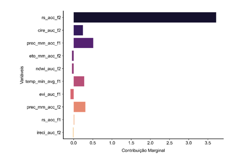
The ranking of the 38 biophysical and agrometeorological characteristics via mRMR (Figure 1) indicated solar radiation in the F2 window as the one with the highest informational relevance. However, the VIF evaluation revealed severe multicollinearity among the 10 pre-selected variables, with solar radiation in F2 presenting a VIF of 84.36. After four rounds of exclusion, six remaining variables with low collinearity were selected: IRECI in F2 (VIF = 1.28), EVI in F1 (VIF = 1.65), solar radiation in F1 (VIF = 1.87), precipitation in F1 (VIF = 2.10) and in F2 (VIF = 2.88), and reference evapotranspiration in F2 (VIF = 2.92).
Figure 1. Ranking of the ten pre-selected variables via mRMR
Source: Original survey data.
Fixed Effects: M6
The insertion of the six selected variables into model M5, centered on the grand mean, was performed by the Forward Stepwise procedure (Table 5). The biophysical index IRECI (F2) contributed the most, promoting a reduction of 9.829 points in the BIC. Subsequent additions resulted in decreasing marginal reductions, culminating with precipitation (F1). In total, the inclusions reduced the BIC from 247.267 to 235.774, resulting in model M6.
Table 5. Iterative inclusion of biophysical and agrometeorological variables via Forward Stepwise procedure (M6).
| Step | Added Variable | Logarithmic Likelihood | LRT | BIC | ΔBIC |
|---|---|---|---|---|---|
| M5 | -123.551 | < 0,001 | 247.267 | ||
| 1 | ireci_auc_f2_cent | – 118.632 | < 0,001 | 237.438 | 9.829 |
| 2 | rs_acc_f1_cent | – 118.354 | < 0,001 | 236.893 | 545 |
| 3 | evi_auc_f1_cent | – 117.927 | < 0,001 | 236.050 | 843 |
| 4 | prec_mm_acc_f2_cent | – 117.853 | < 0,001 | 235.911 | 139 |
| 5 | eto_mm_acc_f2_centroid | – 117.799 | < 0,001 | 235.815 | 96 |
| 6 | prec_mm_acc_f1_cent | – 117.774 | < 0,001 | 235.774 | 41 |
Source: Original survey data. Note: ΔBIC calculated with respect to the immediately preceding iterative step. The suffix _cent indicates that the variable was centered on the grand mean.
This structuring resulted in the study’s greatest explanatory gain (Table 6). The simultaneous inclusion of biophysical and agrometeorological predictors reduced residual variance by 26.1% and crop variance by 90.7%. This decrease indicated that the interannual fluctuation in productivity was almost entirely explained by the fixed-effect predictors, restricting the random effect of the crop to 1.43% of the model’s total variance. This behavior corroborates the premise that the temporal variability of productivity is predominantly governed by agrometeorological conditions and the crop’s biophysical response in each cycle (Marin et al., 2008; Silva, M.G.S. et al., 2022).
Table 6. Evolution of the statistical adjustment of the model in the addition of fixed effects (M6).
| Model | σ²t (plot) | σ²v (variance) | σ²s (crop) | σ²e (residuals) | BIC | ΔBIC |
|---|---|---|---|---|---|---|
| M5 | 92,53 | 48,85 | 31,89 | 177,27 | 247.267 | 3.659 |
| M6 | 42,40 | 29,66 | 2,95 | 130,91 | 235.774 | 11.493 |
Source: Original survey data. Note: ΔBIC calculated relative to the previous model.
Random Slopes: M7
The final structuring step evaluated the culture’s sensitivity to specific variables by including random slopes for the variety context. The Forward Stepwise strategy identified the NDRE index in F1 and the vapor pressure deficit in F2 as the two variables that met the validation criteria (Table 7).
Table 7. Summary of valid iterations for the inclusion of random slopes.
| Round | Random Effect Predictor | Fixed Effect Replaced | ΔBIC | Percentage Change (%) |
|---|---|---|---|---|
| 1 | vpd_kpa_avg_f1_cent | eto_mm_acc_f2_centroid | 82 | 2,37 |
| 1 | vpd_kpa_avg_f2_cent | eto_mm_acc_f2_centroid | 282 | 4,46 |
| 1 | ndre_auc_f1_cent | evi_auc_f1_cent | 378 | 3,22 |
| 1 | ndre_auc_f2_cent | ireci_auc_f2_cent | 157 | 3,74 |
| 2 | vpd_kpa_avg_f1_cent | eto_mm_acc_f2_centroid | 121 | 1,99 |
| 2 | vpd_kpa_avg_f2_cent | eto_mm_acc_f2_centroid | 223 | 4,06 |
Source: Original survey data. Note: ΔBIC calculated in relation to the respective baseline model. Table only with the evaluated predictors that surpassed the validation criteria.
Within the scope of fixed effects, the insertion of these new slopes required the prior removal of EVI (F1), reference evapotranspiration (F2), and precipitation (F1) due to multicollinearity and loss of statistical significance (p = 0.062). The analysis of random effects in model M7 evidenced the genotype-environment interaction. The slopes of NDRE in F1 and vapor pressure deficit in F2 retained 2.41% and 4.06% of the total variance, respectively. These predictors acted as quantitative indicators of genetic heterogeneity, with the dynamics of NDRE in F1 reflecting canopy closure and initial nitrogen uptake efficiency (Shendryk et al., 2020), and sensitivity to vapor pressure deficit in F2 signaling tolerance to hydric stress (Inman-Bamber and Smith, 2005). Modeling this interaction reduced the residual variance to 125.79 (t ha⁻¹)² and attenuated the crop variance to 1.85 (t ha⁻¹)², representing 0.86% of the total variance (Table 8).
Table 8. Evolution of the statistical adjustment of the model in the addition of random slope effects (M7).
| Model | σ²t (plot) | σ²v (variance) | σ²v0 | σ²v1 | sigma squared v two | σ²w (harvest) | σ²e (residuals) | BIC | ΔBIC |
|---|---|---|---|---|---|---|---|---|---|
| M6 | 42,40 | 29,66 | 2,95 | 130,91 | 235.774 | 11.493 | |||
| M7 | 45,94 | 31,00 | 5,20 | 8,74 | 1,85 | 125,79 | 235.032 | 742 |
Source: Original survey data. Note: ΔBIC calculated relative to the previous model. σ²v0: variance of the random intercept of variety; σ²v1: variance of the random slope of NDRE (F1); σ²v2: variance of the random slope of VPD (F2).
Validation and Performance Evaluation of Models
To quantify the evolution of predictive power, the M3 model served as a comparative baseline (Table 9). Its Conditional Pseudo-R² (R²c) indicated that the contexts of plot, variety, and crop explained 45.7% of the total productivity variance, with an MAE of 12.63 t ha⁻¹ and RMSE of 15.88 t ha⁻¹.
Table 9. Predictive performance evaluation metrics and information criteria of the multilevel models adjusted for TCH estimation.
| Model | BIC | LRT | R²m | R²c | MAE (t ha⁻¹) | RMSE (t ha⁻¹) |
|---|---|---|---|---|---|---|
| M3: Cross-validation | 265.139 | < 0,001 | 0,000 | 0,457 | 12,63 | 15,88 |
| M4: with Agronomic Control | 250.926 | < 0,001 | 0,475 | 0,664 | 10,33 | 13,26 |
| M5: with Age Control | 247.267 | < 0,001 | 0,521 | 0,730 | 9,25 | 11,91 |
| M6: with Fixed Effects | 235.774 | < 0,001 | 0,709 | 0,802 | 7,89 | 10,48 |
| M7: with Random Slope | 235.033 | < 0,001 | 0,713 | 0,811 | 7,72 | 10,24 |
Source: Original survey data
The addition of agronomic controls and crop age (M4 and M5) increased the marginal explanatory capacity. M5 captured 52.1% of the variance through its fixed effects (R²m), raising the global explanation (R²c) to 73.0% and reducing the RMSE to 11.91 t ha⁻¹. The greatest marginal gain occurred in M6, with the inclusion of biophysical and agrometeorological variables, which raised the variance explained by fixed effects (R²m) to 70.9% and reduced the MAE to 7.89 t ha⁻¹.
The inclusion of random slopes in model M7 consolidated the genotype-environment interaction, validated by LRT (p < 0.001) and with the lowest BIC (235.033). The final model achieved an MAE of 7.72 t ha⁻¹ and RMSE of 10.24 t ha⁻¹, with a global explanation (R²c) of 81.1%. The difference of 9.8% between R²c and R²m (0.713) represented the variability attributed to plot, variety, and harvest contexts, justifying the multilevel approach (Gelman and Hill, 2006).
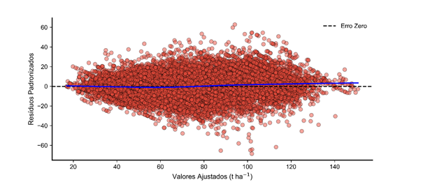
The verification of the assumptions of homoscedasticity and linearity of model M7, through graphical analysis, showed that the dispersion of standardized residuals did not reveal severe funneling patterns (Figure 2), validating the constancy of variance. The non-parametric trend line remained close to zero, attesting to the absence of systematic bias in the predictions (Zuur et al., 2009).
Figure 2. Scatter plot of standardized residuals versus fitted values for homoscedasticity diagnosis of model M7.
Source: Original survey data.
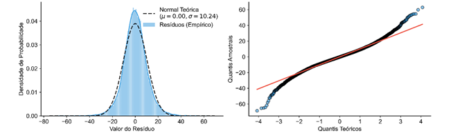
The distribution of residuals showed adherence to theoretical quantiles in the central portion (Figure 3), although with deviations in the tails (leptokurtosis). Such deviations do not preclude statistical inference in multilevel models, given the asymptotic robustness guaranteed by the Central Limit Theorem given the expressive sample size (Zuur et al., 2009).
Figure 3. Probability density distribution and quantile-quantile plot for checking the normality of the residuals of model M7.
Source: Original survey data.
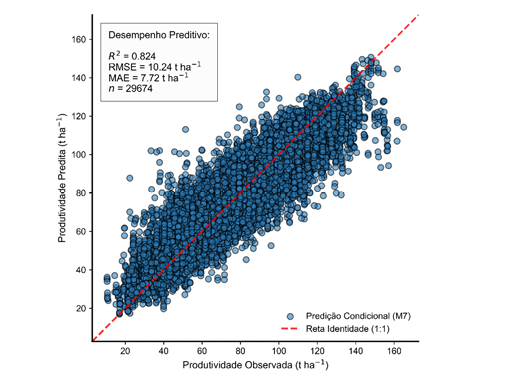
In the evaluation of predictive performance, the dispersion of estimates (Figure 4) validated the model’s explanatory capacity, showing high adherence to the identity line. The global error metrics (MAE = 7.72 t ha⁻¹ and RMSE = 10.24 t ha⁻¹) and the coefficient of determination (R²predictive = 0.824) attested to the practical adequacy of the model.
Figure 4. Relationship between observed sugarcane productivity (TCH) and the values predicted by model M7.
Source: Original survey data.
Compared to Machine Learning techniques, the results obtained were equivalent to those of Random Forest algorithms, which registered RMSE between 11.70 and 15.56 t ha⁻¹ and MAE of 4.57 to 7.53 t ha⁻¹ (Amaro, 2023; Bocca and Rodrigues, 2016). The multilevel approach presented equivalent predictive accuracy, with the inferential advantage of allowing direct interpretation of agronomic parameters, quantifying the variance partition and expliciting the genotype-environment interaction.
The extraction of fixed effects coefficients revealed the estimated magnitude of management, environment, climate, and biophysical state impacts (Table 10). The global intercept was 98.06 ± 1.35 t ha⁻¹, representing the theoretical average basal productivity of a first-ratoon sugarcane field (plant cane), in the highest potential environment (environment A), under continuous predictors centered on their respective global means.
Table 10. Parameter estimates of fixed effects of model M7 for predicting productivity (TCH).
| Parameter | Global Average | Estimate ± SE | CI (95%) | t | p-value |
|---|---|---|---|---|---|
| baseline average productivity | 98,06 ± 1,35 | 95,41; 100,70 | 72,73 | < 0,001 | |
| Management Controls | |||||
| 2nd cutoff | -8,99 ± 0,29 | -9,55; -8,42 | -31,11 | < 0,001 | |
| 3rd cut | -18,82 ± 0,30 | -19,40; -18,25 | -63,87 | < 0,001 | |
| 4th cut | -23,60 ± 0,31 | -24,21; -22,99 | -76,19 | < 0,001 | |
| 5th cut | -25,00 ± 0,34 | -25,67; -24,32 | -72,62 | < 0,001 | |
| 6th cut | -26,91 ± 0,42 | -27,73; -26,09 | -64,44 | < 0,001 | |
| 7th cut | -28,94 ± 0,65 | -30,22; -27,66 | -44,42 | < 0,001 | |
| environment B | -4,22 ± 0,57 | -5,35; -3,10 | -7,35 | <0,001 | |
| C environment | -9,69 ± 0,58 | -10,83; -8,55 | -16,61 | < 0,001 | |
| environment D | -12,27 ± 0,59 | -13,43; -11,12 | -20,81 | < 0,001 | |
| environment E | -15,32 ± 0,63 | -16,56; -14,08 | -24,18 | < 0,001 | |
| Continuous Predictors | |||||
| age (days) | 387 | 0,079 ± 0,001 | 0,076; 0,081 | 62,69 | < 0,001 |
| NDRE (F1) | 25,73 | 0,464 ± 0,053 | 0,360; 0,568 | 8,74 | < 0,001 |
| IRECI (F2) | 94,66 | 0,292 ± 0,004 | 0,286; 0,299 | 82,67 | < 0,001 |
| vapor pressure deficit (F2) | 1,32 | -11,40 ± 2,75 | -16,79; -6,00 | -4,14 | < 0,001 |
| precipitation (F2) | 527,79 | 0,007 ± 0,001 | 0,006; 0,008 | 10,08 | < 0,001 |
| solar radiation (F1) | 1.899,53 | -0,015 ± 0,001 | -0,015; -0,014 | -35,35 | < 0,001 |
Source: Original survey data. Note: SE = Standard Error; CI = Confidence Interval; t = t-statistic; Continuous variables centered on the grand mean.
The succession of cycles showed a non-linear decrease in productivity, with the second cut resulting in an estimated reduction of 8.99 ± 0.29 t ha⁻¹, and the seventh cut in a penalty of 28.94 ± 0.65 t ha⁻¹. The transition from environment A to E (restrictive) subtracted 15.32 ± 0.63 t ha⁻¹ from the average basal productivity. Regarding crop age, the model estimated a gain of 0.079 ± 0.001 t ha⁻¹ for each additional day, indicating that an increment of 1 t ha⁻¹ demands approximately 13 days in the cycle.
In the biophysical scope, NDRE (F1) presented a coefficient of 0.464 ± 0.053 t ha⁻¹, validating its relationship with initial nitrogen uptake efficiency (Shendryk et al., 2020) and canopy closure speed (Dong et al., 2019). IRECI (F2) corroborated the prediction of vegetative growth with a coefficient of 0.292 ± 0.004 t ha⁻¹, ratifying the Red-Edge band’s capacity to quantify biomass with resistance to optical saturation in dense canopies (Dong et al., 2019). For this predictor, a unit gain in productivity is associated with an average increase of 0.023 in the index during the F2 window.
Among the agroclimatological variables, vapor pressure deficit (F2) stood out as a restrictive factor, with a coefficient of -11.40 ± 2.75 t ha⁻¹, indicating that hygrometric stress restricts carbon assimilation (Inman-Bamber and Smith, 2005). In contrast, precipitation (F2) showed a coefficient of 0.007 ± 0.001 t ha⁻¹, suggesting that a supplementary volume of 143 mm (28.6 mm month⁻¹) is necessary for the same productive increment. Solar radiation in F1 showed a negative coefficient of -0.015 ± 0.001 t ha⁻¹, confirming its function as a proxy for thermohygrometric stress on excessively clear days, which accelerate dehydration (Inman-Bamber and Smith, 2005).
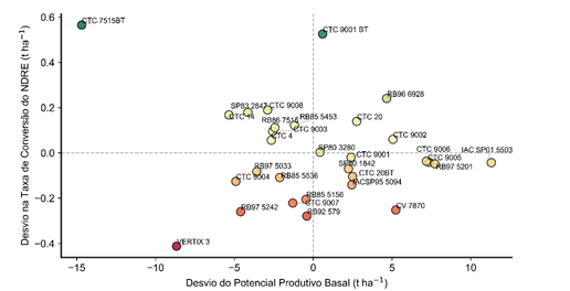
The random slopes showed varietal heterogeneity. The IAC SP01 5503 variety presented the highest positive intercept deviation (11.31 t ha⁻¹), raising its reference level to 109.37 t ha⁻¹ under reference conditions. In contrast, CTC 7515BT registered a severe negative deviation (-14.69 t ha⁻¹), indicating a lower basal productive ceiling. Figure 5 illustrates the relationship between basal productive potential and varietal response to NDRE in F1.
Figure 5. Relationship between basal productive potential and varietal response to NDRE in F1.
Source: Original survey data.
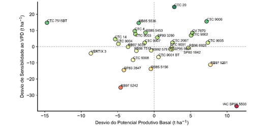
In the window of high vegetative growth (F2), the evaluation of vapor pressure deficit mapped the vulnerability profile to hygrometric stress. IAC SP01 5503 demonstrated extreme sensitivity, with BLUP of -36.74 t ha⁻¹, resulting in a penalty of 48.14 t ha⁻¹ for each 1 kPa increase in this deficit (Figure 6), which suggests its inadequacy for areas with water deficiency. In contrast, genotypes such as CTC 20 exhibited high physiological robustness, with a strongly positive random slope (24.49 t ha⁻¹), nullifying the global penalty imposed by thermohydric stress and justifying its strategic allocation in more restrictive environments.
Figure 6. Relationship between basal productive potential and varietal sensitivity to vapor pressure deficit in F2.
Source: Original survey data.
In summary, multilevel modeling with cross-classification proved to be a robust approach for predicting sugarcane productivity, allowing for the decomposition of variance into spatial, genetic, and temporal components. The integration of biophysical and agrometeorological predictors captured the crop’s phenological dynamics, and the final model achieved predictive accuracy comparable to Machine Learning algorithms while maintaining the interpretability of agronomic coefficients. The results indicated the significant influence of cutting number, production environment, crop age, and biophysical and agrometeorological variables on productivity, in addition to highlighting varietal heterogeneity in response to factors such as NDRE and vapor pressure deficit.
4. Conclusion
Multilevel modeling with cross-classification proved to be a robust analytical approach and methodologically adequate for predicting sugarcane productivity in the southeastern region of Mato Grosso do Sul, covering the harvests from 2019/2020 to 2023/2024. It was found that the approach adequately partitioned spatial, genetic, and temporal variance, successfully quantifying genotype-environment interaction. The final adjustment with random slopes (M7) explained 81.1% of the total variance and achieved a Root Mean Squared Error of 10.24 t ha⁻¹. The 9.8% difference between the marginal and conditional Pseudo-R² evidenced the relevant explanatory gain generated by cross-classification, matching its predictive performance to the accuracy reported by Machine Learning algorithms. This approach, however, maintained the parametric rigor and interpretability of agronomic predictors, such as cutting number, production environment, crop age, biophysical indices (NDRE and IRECI), and agrometeorological variables (vapor pressure deficit, precipitation, and solar radiation). The main contribution lies in offering a transparent and robust analytical tool for productivity estimation and planning in the sugarcane sector, allowing for a detailed understanding of the influence of contextual factors and varietal heterogeneity.
Despite the attested robustness, the study presents limitations inherent to the scope of empirical models. The extrapolation of inferences is restricted to the varietal portfolio and the specific edaphoclimatic conditions of the study area. Deviations were observed in the distribution of residuals in the extreme tails, signaling the occurrence of phenological anomalies, omitted agrometeorological variables, or complex interactions that the linear parametric structure could not fully absorb. For future developments, it is suggested to expand the sampling domain, incorporate spatial autocorrelation structures to capture the dependence between nearby plots, and transition to Generalized Additive Mixed Models (GAMM). These initiatives will allow for refining the mapping of climatic extremes and consolidating the technique as a valuable analytical intelligence tool in the sugarcane-energy sector.
Bibliographic References
Associação de Produtores de Bioenergia de Mato Grosso do Sul [BIOSUL]. 2024. Mapa da Bioenergia de Mato Grosso do Sul. Disponível em: . Acesso em: 20 mar. 2025.
Avilez, A.Μ.Α.; Hernandez, F.B.T.; Bispo, R.C.; Giovanelli, L.B. 2018. Necessidade hídrica da cana-de-açúcar no Noroeste Paulista. Irriga 1(1): 171-188.
Empresa de Pesquisa Energética [EPE]. 2024a. Balanço Energético Nacional 2024: Ano base 2023. EPE, Rio de Janeiro, RJ, Brasil.
Empresa de Pesquisa Energética [EPE]. 2024b. Nota técnica: Análise de conjuntura dos biocombustíveis – ano 2023. EPE, Rio de Janeiro, RJ, Brasil.
Manzatto, C.V.; Assad, E.D.; Bacca, J.F.M.; Zaroni, M.J.; Pereira, S.E.M. 2009. Zoneamento agroecológico da cana-de-açúcar: expandir a produção, preservar a vida, garantir o futuro.
Article originating from the Course Conclusion Work of the Specialization in Data Science and Analytics of the MBA USP/Esalq
To learn more about the course, click here and access the MBX Academy platform