Performance of Machine Learning Models in the Selection of Brazilian Stock Exchange Stocks

Masalskas, Gabriel Fernandes; Janes, Ricardo

doi:10.22167/2675-6528-202602221

Article

September 10, 2026

Performance of Machine Learning Models in the Selection of Brazilian Stock Exchange Stocks

Gabriel Fernandes Masalskas; Ricardo Janes

DOI: 10.22167/2675-6528-202602221

Article derived from a Final Course Work (TCC), with content based on the student’s original work and adapted to the editorial format of the Revista E&S with the support of the ResumeAI tool, an artificial intelligence solution developed by the Pecege Institute for textual synthesis and organization.

Summary

The Brazilian stock market, characterized by high volatility and liquidity constraints, poses challenges to the application of machine learning models in return prediction and investment strategy construction. The study compared the predictive and economic performance of machine learning models and traditional statistical methods in estimating future returns and forming portfolios based on asset ranking. Historical data from B3 stocks were used, with technical and financial variables derived from prices and volume. Linear models (Linear Regression, Ridge, LASSO, Elastic Net), ensemble models (Random Forest, XGBoost, LightGBM), and a neural network (Multilayer Perceptron) were evaluated. Predictive evaluation was performed using error metrics on a test set, and economic evaluation through backtesting of long-only strategies, with operational costs based on turnover for gross and net return analysis. The results revealed low predictive capacity across all models, with negative R² and high errors. Although marginal differences in predictions generated variations in economic performance, these were of low magnitude and unstable. The LightGBM model achieved the best economic performance, but with limited gains compared to the benchmark after including operational costs. No consistent evidence of superior risk-adjusted return generation was observed.

Keywords: machine learning; backtest; stock market; return prediction; asset selection.

1. Introduction

The Brazilian stock market, traded by B3 S.A. – Brasil, Bolsa, Balcão (B3), presents particularities that differentiate it from developed markets, imposing specific challenges for the application of machine learning models in return prediction and investment strategy construction. Understanding its dynamics is fundamental for investors and researchers seeking to optimize performance and risk management in a highly complex environment.

Among the distinctive characteristics of the Brazilian market, higher volatility, lower liquidity depth, and higher operational costs stand out. Comparative studies confirm that emerging markets, such as Brazil, tend to exhibit greater sensitivity to volatility shocks and lower structural liquidity compared to mature markets. Vartanian (2023), for example, identified Brazil among the most volatile markets during periods of instability. De Carvalho (2021) highlighted a significant liquidity premium in B3 stocks, while Brito (2024) demonstrated that the relationship between liquidity and volatility in the national market is accentuated during crises. Additionally, Benetti et al. (2007) emphasized that operational and tax costs in the Brazilian stock market remain higher than those observed in developed countries. These structural particularities make Brazil a challenging environment for the implementation of quantitative strategies.

In this context, machine learning (ML) emerges as a promising tool for analyzing and predicting returns of variable income assets. Recent literature already demonstrates significant advances in the application of ML in finance. Arismendi-Zambrano et al. (2023) showed that ML methods based on penalized regressions are capable of predicting intraday returns in the Brazilian market, generating strategies with performance adjusted for transaction costs superior to linear benchmarks. In the field of fund management, the CFA Society Brazil (2024) applied XGBoost to distinguish managers, finding that portfolios formed based on the model’s predictions presented a better risk-return ratio. Felizardo and Pinto (2019) also evaluated artificial neural network architectures in predicting returns of Brazilian stocks, demonstrating gains in assertiveness compared to linear approaches, although they highlighted the sensitivity of performance to hyperparameter calibration. Additional evidence (Henrique et al., 2019) indicates the potential of non-linear models, such as Support Vector Regression, in predicting prices and returns of financial assets in Brazil, despite limitations associated with model stability and generalization.

Despite these advances, relevant gaps persist in the national literature. Most works focus on high-frequency predictions or fund analyses, with rare research systematically comparing different families of ML models, such as Random Forest, boosting (XGBoost, LightGBM), and neural networks, in asset recommendation contexts in the stock market. Furthermore, few studies incorporate operational elements of Brazilian reality, such as transaction costs, slippage, and effective liquidity, in their backtests and temporal validations. This lack of comprehensive evaluation prevents a complete assessment of the practical and economic viability of ML-based strategies in the local market.

The application of ML in the Brazilian financial market is therefore in a promising stage, but still lacks approaches that reconcile predictive robustness and operational viability. As highlighted by De Prado (2018) and Gu, Kelly, and Xiu (2020), the success of ML models in finance depends not only on statistical performance but also on the ability to generate economically useful and feasible predictions. In the national context, this discussion becomes particularly relevant due to liquidity constraints and trading costs, which can render profitable strategies unfeasible in simulations. Thus, it becomes necessary to develop studies that comparatively and reproducibly evaluate the performance of different ML algorithms in asset recommendation strategies in the Brazilian stock market, using risk-adjusted metrics such as the Sharpe ratio, as well as drawdown and volatility measures. In particular, understanding which models offer the best trade-off between performance and operational viability is a relevant contribution to both academic research and professional practice. Therefore, this work aims to compare the predictive and economic performance of machine learning models and traditional statistical methods in estimating future returns and constructing ranking-based investment strategies in the Brazilian stock market.

2. Material and Methods

This work evaluated the predictive capacity and economic utility of different machine learning models and traditional statistical methods applied to the Brazilian stock market. The analysis was conducted using historical adjusted price data of stocks traded on B3, covering an unbalanced panel of assets.

Definition of the investable universe and data treatment

The study used historical data of adjusted stock prices traded on B3, obtained from the platform “Market Data – Stocks listed on B3” and collected via the Python yfinance library (Yahoo Finance). The price series corresponded to adjusted closing prices (“adjusted close”), which incorporate corporate events such as dividends and stock splits, ensuring temporal consistency of returns.

From the initial set of assets, eligibility and sequential filtering criteria were applied to define the investable universe. These criteria included historical data availability, price consistency, minimum liquidity (traded financial volume), and exclusion of incomplete or inconsistent series, as detailed in Table 1.

Table 1. Steps for defining the investable universe

Step	Description
Initial base	Stocks listed on B3
Data collection	Assets with history available in the provider
Quality filter	Exclusion due to price and volume inconsistencies
Minimum history	Exclusion of insufficient series
Liquidity	Monthly selection of the 50 most liquid assets
Final universe	Dynamic panel of eligible assets

Source: Original survey data

The daily data were aggregated for monthly periodicity, using the last available closing price in each month. Additionally, in each period, the 50 most liquid assets (based on daily traded financial volume) were selected to form a dynamic investable universe, reflecting the market’s operational reality.

Definition of the target variable

The variable of interest was the future monthly logarithmic return of each asset, calculated from the monthly closing prices, according to Equation 1:

r_t+1 = ln(P_t+1 / P_t) (1)

where: r_t+1 is the logarithmic return in period t+1; P_t+1 is the closing price in period t+1; and P_t is the closing price in period t. This return was associated with period t (shift), so that predictions made at the end of month t referred to the return observed in month t+1. The problem was formulated as a supervised regression task to estimate continuous future returns. The economic evaluation of the strategies was based on simple returns.

Construction of the explanatory variables and models

The explanatory variables included lagged returns, volatility measures, trend indicators, and price- and volume-based technical metrics, as detailed in Table 2.

Table 2. Explanatory variables used in the modeling

Group	Variable	Description
Returns	log_return_1d	Daily logarithmic return
Returns	return_5d	5-day cumulative return
Returns	ret_21d	Monthly return
Returns	ret_63d	Quarterly return
Returns	return_252d	Annual return
volatility	vol_21d	Standard deviation of returns (21 days)
volatility	vol_63d	Standard deviation of returns (63 days)
Trend	price_sma21_ratio	Price / 21-day moving average ratio
Trend	price_sma63_ratio	Price / 63-day moving average ratio
Trend	sma_diff_21_63	Difference between moving averages (21d – 63d)
Indicators	rsi_14	Relative Strength Index (14 days)
Indicators	rsi_21	Relative Strength Index (21 days)
Indicators	macd	MACD Indicator
Indicators	macd_signal	MACD signal line
Indicators	macd_hist	MACD Histogram
Risk	ATR_14	Average True Range (14 days)
Liquidity	vol_avg_21d	Average traded volume
Liquidity	vol_med_63d	Average volume (63 days)
Liquidity	vol_fin_med_21d	Average financial volume
Liquidity	vol_fin_med_63d	Average financial volume (63 days)
Liquidity	revenue_proxy	Liquidity proxy
Others	adx_14	Average Directional Index
Others	obviously	On Balance Volume

Source: Original survey data

The variables were calculated daily and aggregated monthly, using the last available observation. All explanatory variables were lagged by one month (t-1) to ensure that the forecasts used only information available up to the end of the previous month.

Representative models of different approaches were selected: linear regressions (Linear Regression, Ridge, LASSO, and Elastic Net), decision tree-based ensemble models (Random Forest, XGBoost, and LightGBM), and an artificial neural network (Multilayer Perceptron – MLP). Table 3 lists the models and their Python implementation libraries.

Table 3. Models used and respective implementation libraries

Model	Library	Implementation
Linear Regression	scikit-learn	LinearRegression
Crest	scikit-learn	Crest
LASSO	scikit-learn	Lasso
Elastic Net	scikit-learn	ElasticNet
Random Forest	scikit-learn	RandomForestRegressor
XGBoost	xgboost	XGBRegressor
LightGBM	lightgbm	LGBMRegressor
Neural Network (MLP)	tensorflow / keras	Sequential (Fully connected)

Source: Original survey data

The explanatory variables were standardized by z-score transformation for scale-sensitive models, while ensemble models were estimated on the original variables. All models were formulated as supervised regression problems to predict continuous future returns. The sample was divided temporally in a sequential manner, with the initial 80% of observations for training and the final 20% for testing, preserving the chronological order of the data.

The predictive evaluation was performed using error metrics (RMSE, MAE, and R²), and the economic evaluation was conducted by a “backtest” on the test set, utilizing metrics such as average return, volatility, Sharpe ratio, and maximum “drawdown”. A benchmark, defined as an equally weighted portfolio of all eligible assets with monthly rebalancing, was used as a reference. To ensure reproducibility, random “seeds” were fixed in the Python (random), NumPy, and TensorFlow libraries.

Construction of ranking-based strategies

The model predictions were used to build “long-only” investment strategies based on “cross-sectional” ranking. Monthly, the 10 assets with the highest predicted return, among the 50 most liquid assets in the investable universe, were selected to form an equally weighted portfolio. The portfolios were fully rebalanced at the end of each month.

Portfolio turnover was measured by the average monthly turnover, which is the proportion of assets replaced between consecutive periods. The strategy return was calculated as the simple average of the realized returns of the selected assets in the subsequent month. Operational costs were incorporated as a simplified estimate, applying a fixed proportional cost of 0.2% per unit of turnover. The net return (r_net) was calculated by deducting this cost from the gross return (r_gross), according to Equation 2:

r_liquidity = r_gross – c * turnover_t (2)

where c is the operational cost (0.2%) and turnover_t is the proportion of assets replaced in period t. The performance of the portfolios was evaluated in the test period in terms of gross and net return, with net return being the main metric for economic comparison. The benchmark, in turn, had no operational costs.

3. Results and Discussion

The interpretation of the results considered the methodological context adopted, including the temporal horizon of the test set period and the simplifications inherent in the backtest, such as the modeling of operational costs based on portfolio turnover (fixed at 0.2%), without the incorporation of additional components like slippage, market impact, and liquidity constraints.

Impact of filters on the asset universe

The application of the eligibility and filtering criteria resulted in a progressive reduction of the initial universe of assets available for analysis. Table 4 presents the selection funnel, detailing the number of remaining assets after each step of the process.

Table 4. Asset universe selection funnel

Step	Number of assets
Initial base (listed actions – CSV)	398
Assets with historical data in the provider	393
After quality filter (price and volume)	150
After minimum history filter	150
Top 50 by liquidity (final sample)	50

Source: Original survey data

A significant reduction in the universe of assets was observed, from 398 to 50, representing an approximate 87% contraction of the initial set. This reduction highlights the high concentration of liquidity in the Brazilian stock market and is consistent with the market structure, where few assets have sufficient trading volume for systematic strategies. The final universe used in the modeling and backtesting predominantly reflects the behavior of more liquid assets. Methodologically, this filtering implies that the results are not directly generalizable to less traded assets, and the dynamic definition of the investable universe influences the composition of portfolios and the benchmark, impacting the comparative evaluation of strategies.

Descriptive statistics of the target variable

Before modeling, the distribution of the target variable, the future monthly logarithmic return, was analyzed to assess its statistical properties and economic plausibility. Table 5 presents the descriptive statistics of the variable.

Table 5. Descriptive statistics of the future monthly logarithmic return

Metric	Value
Observations	3.207
Average	0,0121
Standard deviation	0,1237
Minimum	-0,9252
1%	-0,3462
5%	-0,1661
25%	-0,0538
Median	0,0118
75%	0,0807
Maximum	0,6987

Source: Original research results

The results indicated a distribution characterized by high volatility and long tails, a pattern widely documented in financial literature (Fama and French, 2015; Harvey et al., 2016). The mean close to zero (0.012) and the high standard deviation (0.124) evidenced a low signal-to-noise ratio environment, making it difficult to identify consistent predictive patterns. The presence of extreme values, with minimum returns close to -92% and maximums around 70%, indicated the occurrence of idiosyncratic events and a negative asymmetry in the distribution, characteristic of emerging stock markets. These properties imply modeling challenges, such as sensitivity to outliers and instability in estimates, reinforcing the importance of evaluating strategy performance in a risk-adjusted manner.

Predictive evaluation of the models

The predictive capacity of the models was evaluated by error metrics such as RMSE, MAE, and coefficient of determination (R²), calculated on the test set. The predictions were based on the explanatory variables described in the methodology. Table 6 presents the predictive performance of the models, comparing linear and non-linear approaches.

Table 6. Predictive performance of the models (RMSE, MAE, and R²)

Model	RMSE	MAE	R²
Straight-line	0.1031	0.0754	-0.0571
Crest	0.1031	0.0754	-0.0567
LASSO	0.1029	0.0753	-0.0533
ElasticNet	0.1030	0.0754	-0.0547
RandomForest	0.1017	0.0742	-0.0297
XGBoost	0.1074	0.0792	-0.1476
LightGBM	0.1121	0.0831	-0.2503
MLP	0.1244	0.0943	-0.5391

Source: Original research results

All models showed low predictive power on the test set, with negative coefficients of determination in all specifications, indicating that their predictions are, on average, inferior to a naive strategy based on the historical average of returns. The differences between models in terms of RMSE and MAE were relatively small, with no evidence of consistent superiority of more complex models over linear approaches. Regularized models, such as LASSO and Elastic Net, showed marginally superior performance, while more flexible models, such as Gradient Boosting and neural networks, exhibited worse performance, suggesting possible overfitting. The proximity between RMSE values and the standard deviation of the target variable (Table 5) suggests that the models are unable to explain a significant portion of the variance in returns in a low signal-to-noise ratio environment. The observed differences should be interpreted with caution, given the absence of statistical evidence of superior predictive ability (Giacomini and White, 2006).

Economic evaluation of strategies

Table 7 presents the main economic performance indicators of ranking-based strategies, calculated in the test period, already deducted from the estimated operational costs based on portfolio turnover. Reported are the average monthly return, the monthly geometric return, the annualized return, the return volatility, the Sharpe ratio, the maximum drawdown, and the average monthly turnover, in addition to the final value of a hypothetical investment of R$ 100.

Table 7. Economic performance of strategies by model

Model	Monthly return (%)	Geom. ret. (%)	Annual return (%)	Volume (%)	Sharpe	Maximum Drawdown (%)	Average monthly turnover	R$ 100 total
LightGBM	0,45	0,15	1,76	8,15	0,1920	-28,79	0,5619	103,10
Crest	0,28	0,01	0,10	7,75	0,1249	-31,31	0,4619	100,18
ElasticNet	0,28	-0,01	-0,07	8,01	0,1225	-33,30	0,4429	99,87
Reference Standard	0,13	-0,06	-0,72	6,41	0,0703	-25,34		98,74
LASSO	0,21	-0,10	-1,21	8,29	0,0873	-34,54	0,4143	97,90
Straight-line	0,13	-0,11	-1,31	7,22	0,0621	-30,96	0,4714	97,72
XGBoost	0,24	-0,12	-1,38	8,83	0,0949	-30,93	0,4524	97,60
RandomForest	0,16	-0,18	-2,10	8,42	0,0644	-31,16	0,3476	96,35
MLP	-0,43	-0,62	-7,14	6,30	-0,2365	-35,44	0,6000	87,84

Source: Original research results

The benchmark, an equally weighted passive strategy with monthly rebalancing, served as a reference. The results indicate that the economic performance of ranking-based strategies was generally limited. The LightGBM model showed the best performance, with a positive monthly geometric return and a final value superior to the initial investment. Regularized linear models, such as Ridge and Elastic Net, also exhibited slightly positive geometric returns. However, models like Linear, LASSO, XGBoost, Random Forest, and MLP showed negative geometric returns, indicating a loss of value over time. The difference between average and geometric return reflects the impact of volatility, resulting in negative compound growth for most models, where the variability of returns exceeded the expected average gain. The performance differences between models were small, and Sharpe ratios remained low, indicating that the risk-return relationship of the strategies was unattractive. The economic evaluation window of 21 months is relatively short, implying that the results are sensitive to specific market conditions and limiting the robustness of the conclusions.

Temporal evolution of the strategies’ performance

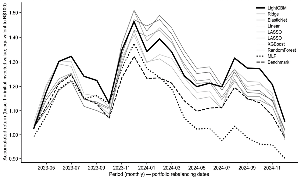
Figure 1 shows the temporal evolution of the accumulated return of ranking-based strategies in the test set period, built from the compound capitalization of the monthly returns of each model, including the benchmark.

Figure 1. Evolution of the accumulated return of strategies based on machine learning models

Source: Original research results

The analysis of Figure 1 shows relevant differences in the performance trajectory between the strategies. The best-performing model presented a relatively more consistent growth trajectory, albeit with episodes of decline, while the worst-performing model exhibited progressive capital deterioration. The benchmark showed intermediate behavior, with a smaller amplitude of variation, reflecting the effect of diversification. The strategies did not follow monotonic growth trajectories, being characterized by alternating cycles of gains and losses. Small differences in model predictions can translate into relevant impacts on accumulated performance, reinforcing the sensitivity of the strategies to the relative ordering of assets. The dispersion between the curves at the end of the period was limited, suggesting that the performance difference stems more from punctual successes than from persistent advantages, aligned with low predictive capacity. The presence of prolonged drawdown periods in almost all strategies highlights the significant associated risk, even in cases of positive final performance, reinforcing the importance of evaluating the temporal dynamics of losses in contexts of high volatility.

Relationship between turnover and economic performance

The incorporation of operational costs, even if simplified, altered the relative ordering of the models, highlighting the importance of accurate modeling of these costs. Table 8 presents the impact of estimated operational costs on the performance of the strategies, including annualized returns and final values before and after cost deduction, as well as metrics associated with portfolio turnover.

Table 8. Impact of transaction costs on strategy performance

Model	Gross annual return (%)	Gross final value (R$)	Average monthly turnover	Total of traded assets	Total cost est. (R$)	Net. ann. ret. (%)	Net final value (R$)
LightGBM	3,15	105,58	0,5619	118	2,36	1,76	103,10
Crest	1,22	102,14	0,4619	97	1,94	0,10	100,18
ElasticNet	1,00	101,75	0,4429	93	1,86	-0,07	99,87
Reference Standard	-0,72	98,74				-0,72	98,74
LASSO	-0,21	99,62	0,4143	87	1,74	-1,21	97,90
Straight-line	-0,19	99,67	0,4714	99	1,98	-1,31	97,72
XGBoost	-0,29	99,49	0,4524	95	1,90	-1,38	97,60
RandomForest	-1,28	97,77	0,3476	73	1,46	-2,10	96,35
MLP	-5,78	90,10	0,6000	126	2,52	-7,14	87,84

Source: Original research results

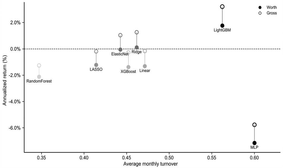
The comparison between gross and net returns shows that the incorporation of costs not only reduces the return but can alter the relative ordering of strategies. Models with superior gross performance may become inferior after cost deduction, especially with high turnover, indicating that evaluation based solely on gross returns can be biased. The average monthly turnover varied between 0.35 and 0.60. Strategies with higher turnover, such as LightGBM and MLP, presented higher accumulated costs. In contrast, models with lower turnover, like Random Forest, had lower return erosion, suggesting that strategy efficiency depends on the interaction between predictive capability and trading intensity. Figure 2 illustrates the relationship between average monthly turnover and net annualized return.

Figure 2. Relationship between average monthly turnover and net annualized return of the strategies

Source: Original research results

Figure 2 does not show a clear monotonic relationship between turnover and performance, indicating that higher levels of turnover do not necessarily imply worse economic performance. However, there is greater dispersion of results among strategies with higher turnover, suggesting that turnover amplifies performance variability by increasing exposure to operational costs. This result indicates that the economic impact of turnover is determined by the interaction between operational costs and the quality of the predictive signal. Strategies with higher relative ordering capacity can offset trading costs, while models with low predictive capacity tend to have their performance deteriorated. The modeling of operational costs is central to the evaluation of machine learning strategies, and the use of simplified proxies, although useful for comparison, may not fully capture real market frictions, overestimating the economic performance of the strategies.

Integrated interpretation of results

The results showed low predictive capacity of the models, with negative R² in the out-of-sample set (Table 6), indicating that they did not outperform predictions based on the historical average of returns. This is consistent with the high volatility and low signal-to-noise ratio of the target variable (Table 5). Despite this limitation, small differences in estimates were sufficient to generate variations in the economic performance of the strategies (Table 7), due to the ranking selection mechanism, where the relative ordering of assets was more relevant than absolute precision. However, these variations were reduced and did not constitute robust evidence of consistent value generation, with the strategies showing net performance close to the benchmark, with occasional gains dependent on the period. The incorporation of operational costs reduced returns and, in some cases, altered the relative ordering of the strategies, highlighting the influence of trading intensity. The relationship between turnover and performance (Figure 2) did not indicate a clear monotonic pattern. The comparison with the benchmark revealed a trade-off between active and passive strategies; although some strategies outperformed the benchmark at certain times, the latter showed lower volatility and more controlled drawdowns (Table 7 and Figure 1), reflecting the effect of diversification. The temporal analysis indicated an absence of persistent superiority among the models, with frequent alternation of performance, suggesting a strong dependence on the time frame. Overall, the evaluated models did not present consistent capacity for generating risk-adjusted returns superior to the benchmark.

4. Conclusion

This work aimed to compare the predictive and economic performance of machine learning models and traditional statistical methods in estimating future returns and constructing ranking-based investment strategies in the Brazilian stock market. It was found that all evaluated models exhibited low predictive capacity on the test set, with negative determination coefficients, indicating that their predictions were, on average, inferior to a naive strategy. Despite marginal differences in predictions, these generated variations in the economic performance of the strategies, albeit of low magnitude and unstable over time. The LightGBM model achieved the best economic performance, but with limited gains compared to the benchmark after incorporating operational costs. No consistent evidence of generating risk-adjusted return superior to the benchmark was observed. The main contribution of the study lies in the systematic evaluation of different machine learning model families in a challenging emerging market, highlighting the importance of operational cost modeling and the limited practical viability of alpha generation strategies in the tested configurations.

The study’s limitations included simplification in operational cost modeling, which did not account for components like slippage and market impact, and the restriction of the asset universe to the 50 most liquid ones, limiting the generalization of results to less traded assets. Additionally, the 21-month economic evaluation window implies sensitivity of the results to specific market conditions. For future studies, it is suggested to implement more robust temporal validation, such as walk-forward approaches, systematic hyperparameter tuning, more realistic modeling of market frictions, and the exploration of different portfolio construction and rebalancing rules, as well as a review of the criteria for defining the investable universe.

Bibliographic References

ARISMENDI-ZAMBRANO, J.; LEONE ALEXANDRE, A.; GENARO, A. Intraday returns forecasting using machine learning: evidence from the Brazilian stock market. SSRN Electronic Journal, 2023. DOI: 10.2139/ssrn.5122977. Acesso em: 9 set. 2025.

BENETTI, C.; DECOURT, R.; RENATO, P. The practice of corporate finance in Brazil and in the USA: comparative survey evidence. São Paulo: ICN Business School; Universidade do Vale do Rio dos Sinos; Catholic University of Santiago de Guayaquil, 2007. Disponível em: https://www.researchgate.net/publication/265454641. Acesso em: 4 nov. 2025.

BRITO, A. D. Instability of returns and liquidity during the Covid-19 pandemic: evidence from the Brazilian stock market. Revista de Administração UFSM, v. 17, n. 2, p. 1–19, 2024. Disponível em: https://periodicos.ufsm.br/reaufsm/article/view/84713. Acesso em: 9 set. 2025.

CARVALHO, G. A. de. Pricing of liquidity risk in the Brazilian stock market. Revista Brasileira de Finanças, v. 19, n. 3, p. 67–94, 2021. Disponível em: https://periodicos.fgv.br/rbfin/article/view/81844. Acesso em: 8 set. 2025.

CFA SOCIETY BRASIL. Using machine learning to separate good and bad equity mutual fund managers: evidence from Brazil. São Paulo: CFA Society Brasil, 2024. Disponível em: https://cfasociety.org.br/wp-content/uploads/2024/09/final_paper.pdf. Acesso em: 14 out. 2025.

DE PRADO, M. L. Advances in financial machine learning. Hoboken: John Wiley & Sons, 2018. Acesso em: 7 fev. 2026.

FAMA, E. F.; FRENCH, K. R. A five-factor asset pricing model. Journal of Financial Economics, v. 116, n. 1, p. 1–22, 2015. DOI: 10.1016/j.jfineco.2014.10.010. Acesso em: 10 jan. 2026.

FELIZARDO, C.; PINTO, A. A study on neural network architecture applied to the prediction of Brazilian stock returns. arXiv preprint, arXiv:1901.09143, 2019. Disponível em: https://arxiv.org/abs/1901.09143. Acesso em: 1 nov. 2025.

GIACOMINI, R.; WHITE, H. Tests of conditional predictive ability. Econometrica, v. 74, n. 6, p. 1545-1578, 2006. DOI: 10.1111/j.1468-0262.2006.00718.x. Acesso em: 19 jan. 2026.

GU, S.; KELLY, B.; XIU, D. Empirical asset pricing via machine learning. The Review of Financial Studies, v. 33, n. 5, p. 2223–2273, 2020. DOI: 10.1093/rfs/hhaa009. Acesso em: 19 jan. 2026.

HARVEY, C. R.; LIU, Y.; ZHU, H. …and the cross-section of expected returns. The Review of Financial Studies, v. 29, n. 1, p. 5–68, 2016. DOI: 10.1093/rfs/hhv059. Acesso em: 19 jan. 2026.

HENRIQUE, B. M.; SOBREIRO, V. A.; KIMURA, H. Stock price prediction using support vector regression on daily and up to the minute prices. Journal of Finance and Data Science, v. 5, n. 1, p. 1–12, 2019. DOI: 10.1016/j.jfds.2018.04.003. Acesso em: 1 nov. 2025.

VARTANIAN, P. R. The VIX index and the volatility of the Latin American and G7 markets. International Journal of Economics and Finance, v. 15, n. 4, p. 1–15, 2023. DOI: 10.5539/ijef.v15n12p25. Acesso em: 1 nov. 2025.

Article originating from the Course Conclusion Work of the Specialization in Data Science and Analytics of the MBA USP/Esalq

To learn more about the course, click here and access the MBX Academy platform

Most recent

Economy, Investments And Banking

October 23, 2026

Educação Financeira, Comportamentos e Vieses na Tomada de Decisão Financeira

October 22, 2026

Challenges and Possibilities of the First School Year of Children with ASD for Teaching Work

October 22, 2026

Consumer Journey in the Decision to Purchase Infoproducts in the Digital Environment

October 22, 2026

Psychosocial Risks and Mental Health at Work in a Banking Institution

October 22, 2026

Digital Observatory of the Amazon: Data Science Applied to the Analysis of Social, Economic, Environmental, and Health Indicators

October 22, 2026

Continuous Learning as a Factor of Organizational Growth in the Perception of Collaborators

October 22, 2026

Statistical Regression in Microgrids for Operational Performance Estimation: Campusgrid Case

October 22, 2026

Forecast of Aggregate Default in the Brazilian Financial System by Sarimax Model with Macroeconomic Variables

October 22, 2026

Stakeholder Engagement Factors in International Technology Transfer to a Public Hospital

A gestão financeira pessoal representa um desafio crescente, influenciada por vieses cognitivos que afetam a tomada de decisão, mesmo em indivíduos com alto conhecimento. O presente estudo analisou a relação entre o nível de educação financeira e a ocorrência de vieses comportamentais na tomada de decisão financeira de adultos residentes no Brasil. Realizou-se um levantamento de campo de natureza aplicada, quantitativa e descritivo-correlacional, por meio da aplicação de um questionário estruturado a 163 respondentes. O instrumento contemplou variáveis sociodemográficas, conhecimento e hábitos financeiros, e situações hipotéticas para identificar vieses cognitivos. Os resultados indicaram que níveis mais elevados de educação financeira associaram-se a melhores práticas de controle financeiro, poupança e investimento, com correlações significativas com renda e escolaridade. Contudo, a presença de vieses comportamentais (ancoragem, aversão à perda, escassez, otimismo/negatividade, viés do presente, status quo, excesso de confiança e contabilidade mental) persistiu mesmo entre indivíduos com maior escolaridade e renda, sem associação estatisticamente significativa com as variáveis sociodemográficas analisadas. Concluiu-se que a educação financeira, embora essencial para a organização e o controle financeiro, não foi suficiente para neutralizar a influência de vieses cognitivos. Sugere-se a incorporação de abordagens comportamentais aos programas de educação financeira.

Palavras-chave: Comportamento financeiro; Economia comportamental; Finanças pessoais; Heurísticas cognitivas; Vieses cognitivos.

October 22, 2026

Challenges and Possibilities of the First School Year of Children with ASD for Teaching Work

The inclusion of children with Autism Spectrum Disorder (ASD) in Early Childhood Education presents significant challenges, given the difficulty of adapting to new environments and the intensity of stimuli. The objective was to analyze the teaching performance in Early Childhood Education in the initial schooling process of children with ASD. A case study was conducted, using narrative interview as a data production technique. The results revealed that the teaching performance was characterized by mediation and affection practices, with the flexibility of routine and the use of playful resources as essential strategies for the child’s development and sensory organization. The importance of the school support professional for the success of the pedagogical work was also highlighted. The child’s integral development was promoted through intentional teaching actions that prioritized environmental adaptation, strengthening of bonds, and attention to the specific needs of ASD. As a contribution, a guide of pedagogical strategies aimed at welcoming children with ASD in public daycare centers was developed.

Keywords: Early Childhood Education; School Inclusion; Teacher Narratives; Inclusive Pedagogical Practices; Autism Spectrum Disorder.

October 22, 2026

Consumer Journey in the Decision to Purchase Infoproducts in the Digital Environment

The expansion of e-commerce and technological transformation have driven the need to understand consumer behavior regarding infoproducts, whose perceived experience has become crucial for professional development. The study aimed to analyze the factors that influenced the purchase decision of infoproducts in the digital environment, considering the stages of the consumer journey. An applied, quantitative, and descriptive research was conducted through a field survey with 100 consumers from Serra Gaúcha. Data collection occurred via a structured questionnaire, using non-probabilistic sampling. The results revealed a qualified audience with strong “mobile-first” behavior. It was found that the availability of detailed information and social approval were the main attraction triggers in the pre-purchase phase. In the transactional and subsequent stages, the minimization of operational friction, the agility of immediate access, and system security proved crucial for conversion and satisfaction, although gaps in human support efficiency were identified. Retention was based on the trust generated by positive past experiences, overcoming the price factor. It was concluded that the infoproduct consumer journey operates as an integrated system, requiring alignment between technological infrastructure, content curation, and support humanization to ensure engagement.

Keywords: E-commerce; Consumer behavior; Consumer experience; Loyalty; Virtual business.

October 22, 2026

Psychosocial Risks and Mental Health at Work in a Banking Institution

Mental health in the workplace is a topic of growing relevance, impacting professional development and employee well-being. A study was conducted to identify aspects and situations that can influence absenteeism levels in a banking institution. The research involved 108 participants and used a structured questionnaire, based on the short version of COPSOQ II by Gonçalves (2021), which contained 45 closed Likert scale questions and two open-ended questions. Data were collected via an online platform and analyzed with a descriptive and quantitative approach. The results revealed a scenario that indicated the need for adjustments in the distribution of activities and in managers’ perception of behaviors and signs of disorders. Important evidence was identified in the participants’ open-ended responses. It was concluded that the study contributed to promoting the perception of a safe environment for mental health in the organization.

Keywords: Absences due to disorders; Professional development; Operational leadership; Medical leave; Mental health.

October 22, 2026

Digital Observatory of the Amazon: Data Science Applied to the Analysis of Social, Economic, Environmental, and Health Indicators

The state of Amazonas faced historical challenges in consolidating the Unified Health System (SUS), stemming from geographical barriers, socioeconomic inequalities, and structural limitations. This study described the development and implementation of a health information geoportal, designed to support monitoring, evaluation, and planning in the Amazonian context. A descriptive case study approach was adopted, based on documentary analysis and secondary data, covering the mapping of functionalities, technical infrastructure, and validation steps of the tool. The Portal was developed with open technologies and integrated multiple national databases, offering interactive dashboards, thematic maps, and a digital document repository. Among the results, highlighted were the georeferenced visualization of key indicators, the possibility of temporal comparative analyses, and the use of the platform in reviewing health plans and redirecting strategic actions. The portal can represent an advance in digital governance and evidence-based management, with potential for replication in other highly complex territories, provided it is accompanied by investments in technological infrastructure, professional training, and inter-institutional coordination.

Keywords: Amazon; Health Evaluation; Digital Health; Health Information Systems.

October 22, 2026

Continuous Learning as a Factor of Organizational Growth in the Perception of Collaborators

The impact of continuous learning and knowledge management on organizational growth was studied in a context of globalization and constant changes. The study’s objective was to analyze employees’ perception of learning culture and its importance for personal and professional development. Data were obtained through an anonymous survey, with a quantitative approach, using a form with “survey” type questions applied to 87 professionals from the technology, health, education, commerce, and services sectors. The results indicated that employees had a positive perception of the contribution of continuous learning to personal and organizational growth, recognizing its benefits for the development of new skills, innovation, and competitiveness. However, it was observed that the incentive for internal knowledge exchange and the offering of practical training still presented moderate levels of agreement. It was concluded that continuous learning significantly contributes to individual and organizational development, suggesting that companies should develop strategic policies for learning focused on new skills, aiming for greater competitive advantage and innovation.

Keywords: Continuous learning; Self-development; Organizational growth; Knowledge Management; Innovation.

October 22, 2026

Statistical Regression in Microgrids for Operational Performance Estimation: Campusgrid Case

A multiple statistical regression model was proposed to estimate the operational performance of UNICAMP’s CampusGrid microgrid, based on internal electrical quantities. The microgrid integrates photovoltaic generation, batteries, and a gas generator. Energy management system data were collected at five-minute intervals over one month. The Operational Reliability Index, defined as the ratio between supplied and demanded energy, was established as the dependent variable. The model was adjusted for the islanded operation mode, evaluating the impact of demand, state of charge, solar generation, and supplied energy. The results revealed high explanatory power, indicating that operational reliability depends on the interaction between supply and demand. It was observed that the nighttime period concentrated the highest rate of partial supply, attributed to the reduction in solar generation. It was concluded that multiple regression offers an interpretable and useful framework for microgrid monitoring and control strategy support.

Keywords: Battery storage; Photovoltaic generation; Reliability Index; Islanded operation; Energy Management System.

October 22, 2026

Forecast of Aggregate Default in the Brazilian Financial System by Sarimax Model with Macroeconomic Variables

Aggregate non-payment in the Brazilian financial system is a crucial indicator of credit risk, the prediction of which is regulated by CMN Resolutions n.° 4.557/2017 and 4.966/2021 for the prospective measurement of expected losses. Aggregate non-payment was modeled and predicted using the SARIMAX model, projecting its trajectory until December 2026 under optimistic, base, and pessimistic scenarios. 164 monthly observations (July/2012 to February/2026) and macroeconomic variables such as unemployment, Selic, IPCA, IBC-Br, and household debt were used. The specification with contemporaneous variables was selected based on information criteria and coefficient stability, and residual diagnostics confirmed statistical adequacy, with a MAPE of 3.12%. Historical non-payment ranged between 4.33% and 7.64%. The estimation identified unemployment (β = 0.2534; p < 0.001) and Selic (β = 0.2128; p < 0.001) as the main positive determinants, with strong temporal persistence (AR(1) = 0.8965). Selic showed increasing correlation with non-payment (r = 0.62 at lag 12), while unemployment demonstrated a contemporaneous effect (r = 0.33). Projections indicated non-payment between 6.30% and 7.98% in December 2026, with a range of 1.68 percentage points, highlighting direct implications for provisioning in financial institutions.

Keywords: Unemployment; Predictive modeling; Monetary policy; Loss provisioning; Time series.

October 22, 2026

Stakeholder Engagement Factors in International Technology Transfer to a Public Hospital

This study described the critical factors perceived for stakeholder engagement in international technology transfer in a public hospital, with a focus on planning. The objective was to describe these conditioning factors, according to the perception of professionals. A single case study was conducted, applying a questionnaire to 25 professionals and using content analysis, complemented by descriptive tabulations. The main obstacles identified were resistance to change (72%), funding (64%), lack of communication (60%), and bureaucracy (40%). Only 28% of respondents recognized the existence of adequate tools for stakeholder management, while 48% denied it and 24% did not know. Exploratory cross-tabulations indicated variations in the assessment of influence according to time of practice, but did not establish causal relationships. Lack of engagement was associated with delays, low adherence, waste of resources, communication failures, compromised knowledge absorption, and risks to patient safety. The conclusions were limited to the perceptions of the researched group and supported preliminary recommendations for intersectoral communication and coordination.

Keywords: Case study; Project Management; Health innovation; Stakeholders; Public sector.

Economy

October 19, 2026

End of the 6×1 scale: what do the numbers allow us to conclude?

Following the promulgation of the end of the 6×1 shift system, the debate on the shorter workday moves to implementation and requires distinguishing social benefits from economic costs. The end of the 6×1 shift system transitioned from legislative discussion to a constitutional change in Brazil. On October 16, 2026, the National Congress promulgated Constitutional Amendment No. 141/2026, originating from Proposal […]

Artificial Intelligence

October 16, 2026

Why study if AI exists?

When answers become easy, learning comes to mean more than just arriving at them. Why do I need to learn this if I can ask an artificial intelligence? This type of question has accompanied education for decades. Why learn an operation if a calculator exists? Why memorize information if it can be found […]

Tax Management

October 15, 2026

Pink tax and the gender of price

How different marketing treatments for men and women are incorporated by consumption taxation Imagine a shelf on which two razors of the same brand and intended for the same purpose are displayed side by side: one has dark packaging and promises strength, precision, and efficiency; the other comes in shades of pink or […]

Health

October 13, 2026

The missing link in health transformation

Why is innovation not enough to drive changes in organizations and health systems Digital transformation has become a strategic priority for health systems worldwide. Electronic health records, artificial intelligence, telemedicine, remote monitoring, and data analysis are now part of the strategic agenda of governments and health organizations. Paradoxically, […]

Marketing

October 09, 2026

Bitcoin or pets: what Artificial Intelligence would not see

A real-life consumer intelligence case shows what gets left out of the brief A few years ago, an American insurance company hired a specialized consumer intelligence firm to answer three questions: The insurer was also considering launching paid insurance in bitcoin. At the time, the consultancy’s workflow was as follows: the analyst created a query […]

School Management

October 06, 2026

The school is not a casino: when trading cards become currency in the playground

Why, for certain students, does school manage to offer so few experiences of achievement? The World Cup is over. Brazil left the competition, the school holidays came, the final was played and the football calendar moved on. It would be reasonable to imagine that, with the end of the tournament and the return to classes, […] would also begin

Energy Transition

September 30, 2026

Renewable energies: the Brazilian advantage

Brazil needs to invest in the capacity to transform natural resources into innovation, productivity, and development. Talking about energy is talking about development. Behind industry, transportation, services, cities, and increasingly artificial intelligence, there is an energy infrastructure that sustains the economy. Understanding a country’s energy matrix is understanding […]

Data Analysis

September 30, 2026

When the data changes, has reality changed?

An analysis of almost 20 million teaching positions-year between 2020 and 2025 shows how changes in population composition and record production can alter the interpretation of historical series Between 2020 and 2025, the number of formal teaching employment positions identified in RAIS (Annual Relation of Social Information), from the Ministry of Labor, […]

Artificial Intelligence

September 28, 2026

Artificial intelligence and the trends

Why do so many people join in on the fun with ChatGPT? I was never the trend person. I still am not. Some pass through my timeline, I see them, I find them interesting but not to the point of trying them out. This was the case, inclusive, with some recent waves of images made by artificial intelligence, like the 80s trend, the one that […]

Tax Management

September 01, 2026

Tax reform and estate planning in the countryside

Efficiency in managing taxes facilitates governance and allows for the organization of family succession. Rural wealth organization has become a strategic measure in light of the tax reform in Brazil, which came into effect this year. The planning of activities and rural wealth management, through tools such as the transition from an Individual to […]

Renata de Gaspari Valdejão Almeida

Artificial Intelligence

August 05, 2026

Inside the company and off the radar: the risks of Shadow AI

According to Microsoft, 75% of professionals already use artificial intelligence at work without company approval. The use of generative artificial intelligence is already part of the corporate routine. Tools like ChatGPT, Copilot, and other platforms help professionals produce texts, analyze data, create presentations, and accelerate tasks in practically all sectors. But this advance […]

Renata de Gaspari Valdejão Almeida

Strategy

July 02, 2026

The future as a competence

Academic interest reinforces the projection of scenarios as an essential tool for decision-making. While some companies are still trying to get the next step right, others are already working with multiple possible futures — and preparing for all of them. But after all, what does it mean to “think about the future”? Is it a trend, a strategy, or a new competence that […]

Renata de Gaspari Valdejão Almeida

Innovation

Technology

May 21, 2026

Agro SP Corridor: innovation, institutional articulation and future

Pecege commands the executive operation of the 400 km ecosystem activities that became known as the Brazilian agro Silicon Valley In 2025, in addition to taking over the management of the Piracicaba Technology Park, the Pecege Institute was also designated to command the executive operation of the State Agribusiness Innovation Corridor activities, the so-called […]

Education

April 27, 2026

How to turn a TCC into a business

New management of the Piracicaba Technology Park offers consulting to MBA graduates The new project director of the Piracicaba Technology Park (PTP), Alexandre Barreto, often says that one of the greatest rewards he has ever had in life was seeing his MBA USP/Esalq students structure companies from their final projects […]

Technology

March 20, 2026

The human repertoire in the age of AI

Critical thinking and creativity are irreplaceable in the work of a marketing professional Artificial Intelligence (AI) is capable of incredible feats, but it does not yet possess the judgment, empathy, intuition, and strategic creativity necessary to do the job of a good marketing professional. In this area, it is important to know how to use the tool to automate […]

Renata de Gaspari Valdejão Almeida

Agribusiness

Innovation

February 23, 2026

ESG as a growth strategy in a cooperative in RS

Santa Clara balances social and environmental responsibility with innovation Founded in 1911 by Italian immigrants in Carlos Barbosa, in the Serra Gaúcha region, Cooperativa Santa Clara is an example that it is possible to balance economic growth with social and environmental responsibility. From a small cheese production company, the organization has evolved into a […]

Renata de Gaspari Valdejão Almeida

Agribusiness

Innovation

January 22, 2026

Brazil free of Foot-and-Mouth Disease: what changes for Brazilian beef?

With a herd of over 200 million head of cattle, the country is currently the leader in exports. Brazil recently received, for the first time, the certification of country free of foot -and-mouth disease without vaccination, conferred by the World Organisation for Animal Health (WOAH). The seal strengthens the country’s position as a reliable supplier of meat for the […]

Renata de Gaspari Valdejão Almeida

Innovation

December 09, 2025

Innovation: the new cycle of the Piracicaba Technology Park

Instituto Pecege assumes management, betting on the creation of new businesses Starting in 2026, Instituto Pecege will assume the management of the Piracicaba Technology Park (PTP). Among its responsibilities will be the administration, operation, maintenance, and expansion of the park, in addition to fostering activities in innovation, entrepreneurship, and science and technology. The choice was made […]

Renata de Gaspari Valdejão Almeida

July 06, 2026

Large-Scale Architecture: DSR-SCRUM Change Management

Mônica Alessandra Guerios; Maria do Carmo Assis Todorov Abstract generated by ResumeAI, an artificial intelligence solution developed by Instituto Pecege focused on synthesis and writing. Architecture and urbanism are configured as essential bases in an increasingly complex and challenging urban space, where the intrinsic connection between social, environmental, and technological issues […]