A comparison between investment strategies using neural networks, statistical methods, and momentum

doi:10.22167/2675-6528-2023116E

Article

February 09, 2024

A comparison between investment strategies using neural networks, statistical methods, and momentum

_{DOI: 10.22167/2675-6528-2023116}
^{E&S 2024, 5: e2023116}

Helcio Haruo Sasaki; Murilo Henrique Tank Fortunato

Artificial intelligence (AI) was born in the mid-20th century and caused two “waves” in the market. The first began in 1950, with Alan Turing^[1]as the main exponent, prevailing until the mid-1980s, amidst advances in computer science. One of the icons of this generation was the development of chess games for computers. A second wave emerged between the 1990s and 2000s, when there was an inversion in the classic programming rule. Until then, it was necessary to explicitly program all possibilities to obtain answers. In “machine learning,” on the other hand, the goal becomes to train the machine for learning, so that it discovers the rule, as illustrated in Figure 1.

Figure 1. Representation of the “machine learning” model before and after

Source: Elaborated by the authors.

Currently, there are already several practical applications for products that use “machine learning”, such as personal assistants, assertive social media marketing tools, improved diagnostic prediction models, and more recently, self-driving cars (notably Tesla’s), AlphaGo (DeepMind’s AI that defeats humans in the game of Go), and ChatGPT (AI capable of creating content), from OpenAI^[2].

Lately, the financial market has begun to incorporate these tools, which have enormous potential for discovering new applications, such as the use of “machine learning” to estimate coffee prices through the “convolutional neural network”^[3] network. The objective of this work was to implement “machine learning” techniques to generate alpha in investments, that is, to perform active management by obtaining returns above the “benchmark”. It is important to mention that, in terms of accuracy, while the machine can achieve high levels of correctness in an image classification model, in the financial market the level of correct predictions is more modest. Robert Mercer, one of the founders of the giant investment management company Renaissance Technologies, once said: “we are right 50.75% of the time, but we are 100% sure 50.75% of the time”^[4].

A portfolio was structured whose resources were equally distributed among four possible investments. The update was monthly and synthesized a 20-year history. Brokerage costs, execution costs, income tax, nor the possibility of short selling the asset (betting on negative asset returns) were considered, as it is not easily implemented for individual investors.

a) Dollar

The benchmark real price for the dollar was measured by the average quote of three existing funds (Santander Fundo Cambial, Itaú Fundo Cambial, and Bradesco Fundo Cambial). Using only the exchange rate variation does not correctly reflect profitability, as there is remuneration on dollar cash.

b) Ibovespa Stocks

Index with the main companies traded on the Stock Exchange, such as: Petrobras, Vale, Itaú, Bradesco, Santander, Banco do Brasil, B3, WEG and Ambev.

c) Two-year pre-fixed interest investment

Average interpolated rate for the two-year maturity, based on the vertices of interbank deposits traded daily on the Stock Exchange (B3). The choice of a generic maturity avoided the need to consider the decay effect of the paper’s maturity. In this analysis, the investment return was considered based on the financial value (PU):

where: PU_i is the present value of the 100 thousand invested; i represents the reference date; du_i represents the business days between i and the generic maturity date; and taxa_i represents the pre-fixed rate negotiated on day i.

d) Five-year fixed-rate investment

Average interpolated rate for the five-year term, based on the vertices of interbank deposits traded daily on the Stock Exchange. The return based on the financial value (PU) was also considered.

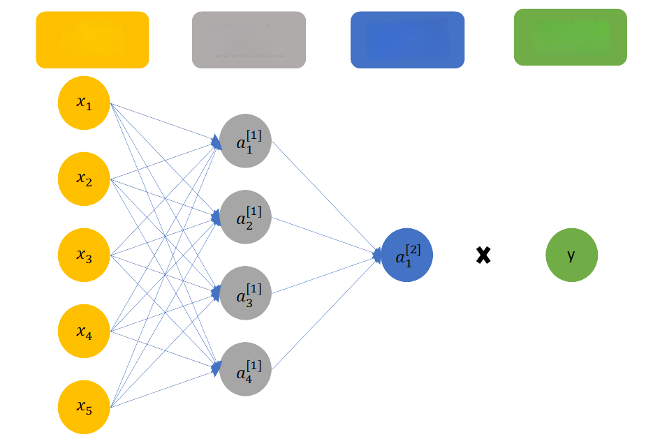
Programming languages — such as R, Java Script, and especially Python — have several neural network packages, like Keras and TensorFlow. According to Chollet^[5], these tools have the advantage of being like building blocks, where one can fit layers of “deep learning” functions and use the “pipeline” to order the flow of information within the structure. However, to gain sensitivity to the rationale and results, a neural network was created from scratch, detailed in Figure 2^[6]:

Figure 2. Diagram of the proposed neural network

Source: Elaborated by the authors.

In this example, there are five input data, a hidden layer (or intermediate layer) and an output layer (or “output” layer) that contains the estimated result. The superscript reference in brackets ([j]) represents the layer of each neuron; in this case, it only varies between 1 (hidden layer) and 2 (output layer). The subscript reference “i” represents the neuron contained in a given layer. In this case, the hidden layer has four neurons, and the output layer contains only one neuron.

The neuron Z_i^[j] can be generically described as the result of the weighted “input” by the weight w^{^–}(“weight”) added to the bias b^[j] (“bias”):

In each of the layers, there is an activation function whose objective is to “turn on” or “turn off” the neuron. This step is important to reduce the risk of error non-convergence, as described in Murray, Abrol and Tanner^[7] and Ovalle^[8], which would make the model unable to find a solution.

In the hidden layer, the hyperbolic tangent activation function tanh was used, using w^[1] to weigh the input data summed with the bias b^[1]. In this way, the intermediate layer neuron attempts to estimate the asset return between a rise (+1) or a fall (-1):

In the output layer a_i^[2] the sigmoid activation function σ was used. Thus, the output layer weights the result of the previous layer a_i^[1] by the weight w^[2] and adds the bias b^[2], thus defining whether it was interesting (+1) or not (0) to invest in the asset:

For the error calculation, the “binary cross entropy” equation ^[9] was used:

where: total error represents the sum of the difference between the estimated value and the realized value; m represents the sample size; a_i^[2] represents the estimated value resulting from the “output layer”; and Y_i represents the observed variable.

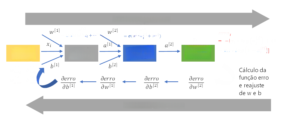
Initially, in the input layer, the values of w^[1] and b^[1] are random values. The result of multiplying the “inputs” by the weight w^[1] is added to the bias b^[1], and the final result passes through a logistic activation function. The information flows to the intermediate layer, where the previous result is multiplied by the new weight w^[2] and is added to the bias b^[2], which are also initially random values. This information flow is called “forward propagation”.

The beauty of the neural network is that, based on the difference between the estimated value and the realized value, a new estimate is made, with a marginal adjustment of the parameters w^[j] and b^[j] to minimize the deviation in the next iteration. This resembles the process of learning through trial and error, which in neural networks is called “backward propagation”^[10].

Figure 3. Information flow within a neural network

Source: Elaborated by the authors.

The correction parameters described in the “backward propagation” of Figure 3 were obtained through the gradient descent optimization method, where the weight correction is defined by:

where: A^[2] represents the expected value in the output layer in matrix; Y represents the realized results in matrix form; and A^_[2]^trepresents the result of the intermediate layer in transposed matrix.

Subsequently, the partial derivative of the error sensitivity with respect to the bias of the output layer, ^b[2], was calculated, represented in matrix form by the mean deviation:

Up to this point, the corrections for the weight and bias of the output layer were calculated. The next step was to calculate the weight and bias adjustment for the hidden layer. The sensitivity of the error with respect to the weight in the intermediate layer, w^[1], was calculated as follows:

where: W^[2]^t represents the weights of the final layer in transposed matrix; and X^t represents the input data in transposed matrix.

Subsequently, the partial derivative of the error with respect to the bias in the intermediate layer was calculated, b^[1]:

where: W^[2]^t represents the weights of the final layer in transposed matrix.

The matrix equations (10) and (11) from the output layer and equations (12) and (13) from the intermediate layer were encoded in Python.

All strategies used 20 years of monthly history, in the period from January 2002 to December 2022.

a) “Long-only” strategy (passive strategy)

The resources were equally divided among four assets: stocks, dollar, two-year interest rates, and five-year interest rates, with no changes during the analysis period.

b) Impetus

Momentum represents the tendency for price increases to perpetuate in the coming periods, just as a fall is generally preceded by further corrections. In this sense, the 2008 Nobel laureates in economics, Fama and French^[12], stated that momentum is a “premier market anomaly”, that is, a strategy that generates above-average returns. Subsequent works have confirmed this anomaly, including in the markets of emerging countries^[11].

Antonacci^[13] went further and proposed a simple but effective strategy on the momentum of assets: if an asset’s return is higher than the risk-free rate, it is applied to that asset for the next period. If the return is lower, it is applied to the risk-free asset.

c) 21-period Momentum

The same logic as the strategy described in the previous item was applied, but a moving average of the returns of the last 21 months was used, a period chosen because it is common in technical analysis.

d) Linear regression [“ordinary least squares (OLS)”]

In this strategy, the coefficients of the lagged linear regression were calculated over a period, as shown in the example for the dollar return:

where: USD_M represents the dollar return in period M; USD_M-1: is the dollar return in period M-1; IBOV_M-1 is the Ibovespa return in period M-1; PRE2_YM-1 represents the return of the investment in two-year fixed-rate interest in period M-1; PRE5_YM-1 is the return of the investment in five-year fixed-rate interest in period M-1; CDI_M-1 is the return of the Interbank Deposit Certificate (CDI) in period M-1; and βs represent the regression coefficients.

As detailed below, the neural network model uses 80% of the data for training. To maintain equality regarding sample size, the same data cut was used to estimate the linear regression coefficients. Thus, for a given month “M”, 80% of the previous observations (17 months) were used to estimate the regression coefficients; the remaining 20% of the observations (four months), as a test sample.

If the estimate of the next period’s return were positive, the resources would be applied to this asset for the following month. Otherwise, the resources would be applied to the risk-free CDI asset.

e) Logistic regression

In the same way that happened with linear regression, the coefficients of logistic regression were estimated based on a moving window of 21 periods: 80% of the sample observations were used to determine the regression coefficients, and the remaining 20% as a test. To define whether the next return would be high (1) or low (0), a cutoff of 0.50 was used as the limit.

f) Neural network

A hidden layer of four neurons with hyperbolic tangent activation and one neuron in the output layer with logistic activation was implemented, as detailed in Figure 2.

The moving window contained the return of the last 21 months; 80% of the previous observations (17 months) were used to estimate the “weight” and “bias” parameters, and the remaining 20% for testing. The learning rate was 0.50, with 1,000 iterations (“epochs”).

If the expected return were positive, the model would apply resources to this asset for the next month. If the expected return were negative, the model would apply resources to the CDI.

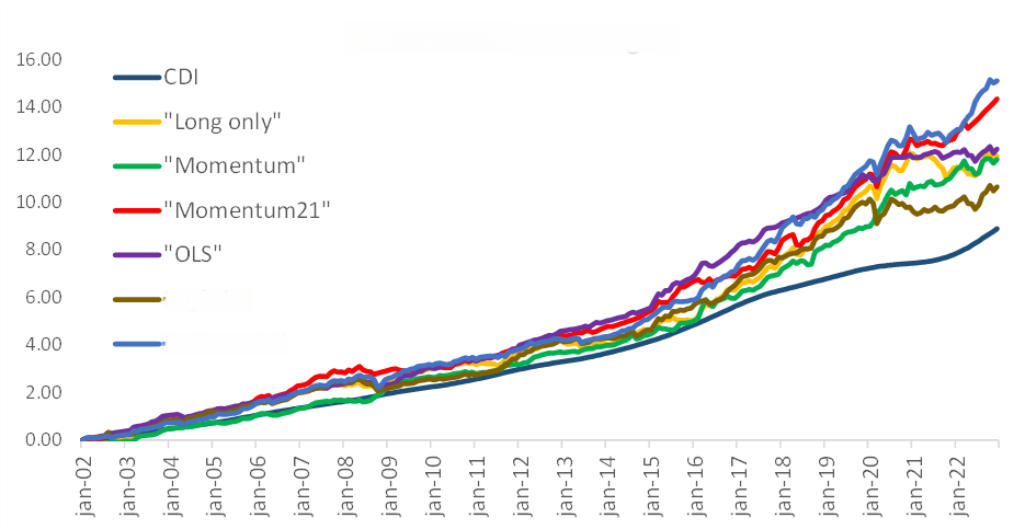
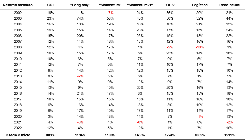
Figure 4 shows the accumulated result of 20 years of the six investment strategies and the “benchmark”, which is the accumulated CDI in the period. Table 1 shows the detailed results by year and strategy.

Figure 4. Monthly accumulated result of the 6 strategies and the accumulated CDI

Source: Elaborated by the authors.

Table 1. Annual result of the different strategies

Source: Elaborated by the authors.

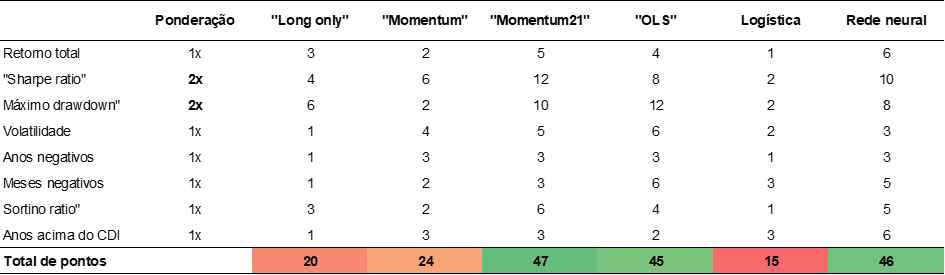
In order to choose the best strategy, eight criteria were evaluated: absolute total return; “sharpe ratio” (return adjusted for volatility); “maximum drawdown” (maximum monthly loss); volatility (standard deviation); number of negative years; number of negative months; “sortino ratio” (return adjusted for downside volatility); and number of years above the CDI.

Table 2. Evaluation measures of the different strategies

Source: Elaborated by the authors.

For each criterion, scores from 1 to 6 were assigned, with 6 being the best and 1 the worst. For the “sharpe ratio” and “maximum drawdown” indicators, there was a double weight weighting, due to their importance for investment evaluation.

Table 3. Ranking of the best strategy (the higher the score, the better)

Source: Elaborated by the authors.

Although the neural network strategy has the best performance, with a return of 1,511% in 20 years, the model that had the best score was momentum with 21 periods, with superior performance in items such as “sharpe ratio”, “maximum drawdown”, “sortino ratio” and volatility.

In the construction of the neural network strategy, variability was observed in the results depending on the “inputs” used, such as learning rate, number of neurons, and number of simulations. Possibly due to lack of model convergence or data “over-fitting”^[14]. Table 5 contains the sensitivity of the result.

Table 5. Risk measures of different neural network strategies

Source: Elaborated by the authors.

The second negative point of neural networks was the lack of sensitivity to how input variables affect the outcome. In the case of a regression, the sensitivity of how explanatory variables affect the outcome can be observed by the regression coefficients, and, in the case of the momentum strategy, the sensitivity can be visualized by the simple average of the last returns.

In any case, all modeling can incur errors caused by the lack of asset liquidity, surprises in the disclosure of indicators, for example, and even by the more intense use of algorithms that operate in the financial market, as “algo trading” (“robots”) can increase the level of noise in prices: if an asset rises unduly due to low liquidity, for example, the computer may notice the price increase and send a buy order, which can further displace the asset’s price.

However, perhaps the main factor distorting prices is the behavioral bias of investors, which tends to oscillate between the extremes of greed and fear^[15], which favored the momentum strategy. The neural network investment strategy with only one hidden layer and one output layer, in turn, presented a very interesting result and surpassed the absolute profitability of the other strategies. However, when considering other performance metrics, such as risk-adjusted return and volatility, the momentum strategy with 21 periods was the winning allocation in the observed 20-year period. This simple strategy also had two advantages over the neural network:

I. simplicity of the decision model, as the choice was for the asset with profitability higher than that of the CDI on average over the last 21 months, given the black box of “machine learning” results, which, because they cannot be reconstructed, demand trust in the model’s “output”;

II. ease in the interpretation and predictability of the decision criterion (an asset that is rising should maintain its trend), compared to the lack of sensitivity to how each variable influences the decision of the neural network model.

It is important to add that the results of the neural networks presented some instability in the simulations depending on the parameters used, which generates insecurity regarding the model’s stability.

Finally, as this field of knowledge is recent, it is important to look closely at improvements in neural network models. At the same time, humility is also necessary to recognize that there may be limitations of “machine learning” models, particularly in the financial market, since investor behavior can sometimes seem more erratic than rational, alternating between moments of euphoria and panic.

References

[1] Turing A. Computing Machinery and Intelligence. MIND A Quartely review of Psycholology and Philosophy. 1950; 59(236): 433-460. Disponível em: https://psycnet.apa.org/doi/10.1093/mind/LIX.236.433. Acesso em: 29 set. 2023.

[2] Harari Y. ‘Sapiens’ author says AI is an alien threat that could wipe us out: ‘Instead of coming from outer space, it’s coming from California. Fortune. 2023. Disponível em: https://fortune.com/2023/09/12/sapiens-author-yuval-noah-harari-ai-alien-threat-wipe-out-humanity-elon-musk-steve-wozniak-risk-cogx-festival/. Acesso em: 29 set. 2023.

[3] Santos J.A.A. Previsão do preço do café arábica: uma aplicação de redes neurais CNN-BLSTM. Research, Society and Development. 2022; 11(3): 1-11. DOI: https://doi.org/10.33448/rsd-v11i3.26101.

[4] Zuckerman G. O Homem que decifrou o Mercado. Rio de Janeiro (RJ): Alta Books; 2020.

[5] Chollet, F. Deep Learning with Python. Shelter Island (NY): Manning; 2018. 384 p.

[6] Verma A. Shallow Neural Net from Scratch Using R. RPubs. 2020. Disponível em: https://rpubs.com/theairbend3r/bin-classification-small-nnet-scratch-r. Acesso em: 29 set. 2023.

[7] Murray M.; Abrol V.; Tanner J. Activation Function Design For Deep Networks: Linearity And Effective Initialisation. Applied and Computational Harmonic Analysis. 2021; 59: 117-154. Disponível em: https://arxiv.org/pdf/2105.07741.pdf. Acesso em: 29 set. 2023.

[8] Ovalle D. The purpose of activation functions in the neural network. Medium. 2020. Disponível em: https://medium.com/@1087/the-purpose-of-activation-functions-in-the-neural-network-be08f81b7c32. Acesso em: 29 set. 2023.

[9] Yathish V. Loss Functions and Their Use In Neural Networks. Medium. 2022. Disponível em: https://towardsdatascience.com/loss-functions-and-their-use-in-neural-networks-a470e703f1e9. Acesso em: 29 set. 2023.

[10] Patel J. Derivation of Backpropagation in Neural Network. Youtube. 2021. Disponível em: https://www.youtube.com/watch?v=URJ9pP1aURo&t=190s. Acesso em: 29 set. 2023.

[11] Blitz D.; Hanauer M.; Vidojevic M. The idiosyncratic momentum anomaly. International Review of Economics & Finance. 2020; 69: 932-957. Disponível em: https://www.sciencedirect.com/science/article/abs/pii/S1059056020300927. Acesso em: 29 set. 2023.

[12] Fama, E.F.; French, K.R. Dissecting Anomalies. The Journal of Finance, 2008. Disponível em: https://doi.org/10.1111/j.1540-6261.2008.01371. Acesso em 29 set. 2023.

[13] Antonacci G. Dual Momentum Investing. Nova York (NY): Mc Graw Hill Education; 2015. 256 p.

[14] Dixon M.; Klabjan D.; Bang J.H. Classification-based financial markets prediction using deep neural networks. Journal Algorithmic Finance. 2017; 6(3-4): 67-77. Disponível em: https://content.iospress.com/articles/algorithmic-finance/af176. Acesso em: 29 set. 2023.

[15] Kindleberger C.P.; Aliber, R.Z. Manias, Panics, and Crashes: A History of Financial Crises. Palgrave MacMillan 7th Edition. 2015.

Como citar

Sasaki H.H.; Fortunato M.H.T. Uma comparação entre estratégias de investimento utilizando redes neurais, métodos estatísticos e momentum. Revista E&S. 2024; 5: e2023116.

Sobre os autores

Helcio Haruo Sasaki, Banco Santander, Avenida Juscelino Kubitschek, 2235 – Vila Olímpia – CEP 04543-011 – São Paulo/SP, Brasil.

Murilo Henrique Tank Fortunato, Instituto de Pesquisa e Educação Continuada em Economia e Gestão de Empresas – Pecege – Rua Cezira Giovanoni Moretti, 580 – Santa Rosa – CEP 13414-157 – Piracicaba/SP, Brasil.

Download link: PDF

Most recent

November 06, 2026

Influence of digital marketing on the consumption of protein supplements and protein-enriched foods

November 06, 2026

Innovation in Operational Management of the Electric Sector with Data Science Support

November 06, 2026

Photovoltaic power generation forecasting through machine learning: a study applied to a plant in the Northeast of Brazil

November 06, 2026

Customer behavior in preparatory courses: RFM segmentation, Markov Chains and supervised learning

November 06, 2026

Optimization of Business Intelligence in Brazilian E-commerce: Fine-Tuning LLMs for Aspect-Based Sentiment Analysis in Customer Reviews

November 06, 2026

Classification of stock returns in Brazil with machine learning and meta-labeling techniques

November 06, 2026

Digital influencers, confidence, and purchase intention in private label cosmetics brands

November 06, 2026

AHP-Gaussian Method in Supplier Selection: Compliance in Public Procurement

November 06, 2026

Positioning of global food brands and consumer perception in the contemporary digital market

The consumption of protein supplements and foods with added protein has grown significantly in recent years, with digital content related to health, aesthetics, and physical performance becoming a relevant part of the routine of Brazilians seeking a disciplined lifestyle. The present study aimed to analyze the consumption behavior of protein supplements and foods, as well as the influence of social media and digital influencers on consumers’ purchasing decisions. An exploratory research was conducted, using an online questionnaire applied to 62 participants via Google Forms, disseminated on Instagram, and a semi-structured interview with the CEO of a supplement brand. The data analysis was quali-quantitative. The results indicated that social media, especially Instagram, played a central role in consumers’ initial contact with brands. The majority of respondents associated the consumption of protein products with a healthy and fitness lifestyle, and considered the influence of digital content creators in stimulating experimentation and purchase. The significant impact of digital marketing and aspirational narratives on consumption behavior was identified, reinforcing the relationship between functional food, social identity, and belonging in the digital environment in the context of protein supplementation and food.

Keywords: Foods with added protein; Consumer behavior; Protein supplement consumption; Digital influencers; Digital marketing.

November 06, 2026

Innovation in Operational Management of the Electric Sector with Data Science Support

The application of data science in the operational management of electric power distribution was investigated with the objective of optimizing processes and strategic decision-making. The study analyzed how predictive algorithms and Business Intelligence dashboards can enhance operational management, aiming to optimize team dispatch, forecast demands, and monitor indicators in real-time for more agile and sustainable decisions. The research was applied in nature and considered historical, geographical, and operational data from EDP São Paulo in São José dos Campos, covering the period from January 2018 to December 2024. The data were processed in a Business Intelligence environment and subjected to machine learning algorithms, such as multiple linear regression and recurrent neural networks, for demand forecasting and fault pattern identification. Additionally, clustering was used to identify critical areas. The results indicated that the integration of forecasting models with real-time operational indicators reduced response time to incidents, increased efficiency in resource allocation, and promoted continuous operational improvement. Recurrent neural networks demonstrated higher accuracy in demand forecasting, and correlation analysis pointed to precipitation as a relevant factor for increased interruptions. The identification of critical areas by clustering allowed for the prioritization of maintenance actions. It was concluded that the adoption of data science methods modernizes the sector, reduces costs, increases reliability, and promotes greater sustainability, providing subsidies for more agile and sustainable decisions in energy management.

Keywords: Predictive algorithms; Business Intelligence; Data science; Energy distribution; Operational management.

November 06, 2026

Photovoltaic power generation forecasting through machine learning: a study applied to a plant in the Northeast of Brazil

The increase in renewable energies in Brazil, especially photovoltaic energy, highlighted the need to improve the prediction of power plant production, due to the high dependence on climatic factors and the consequent variability of electricity generation. Machine learning models were developed and evaluated for predicting the electricity generation of a photovoltaic power plant in Northeast Brazil, analyzing the impact of the progressive inclusion of meteorological, temporal, derived, and lagged variables. Hourly data on energy generation and meteorological variables from official and public databases were used. Three tree-based regression algorithms (Decision Tree, Random Forest, and XGBoost) were implemented in a modeling structured in three phases: meteorological, temporal and cyclical variables, and lags. The results indicated a strong correlation between solar radiation and energy generation. Moderate predictive performance was observed in the initial phases of modeling, with a significant improvement in the third phase, where XGBoost stood out with an R² of 0.898. It was concluded that the inclusion of temporal variables and feature engineering techniques was decisive for improving the predictive capacity of the three models, configuring itself as a strategy for practical applications in the photovoltaic sector.

Keywords: Tree-based algorithm; Meteorological data; Temporal dependence; Feature engineering; Solar farm.

November 06, 2026

Customer behavior in preparatory courses: RFM segmentation, Markov Chains and supervised learning

An analytical architecture was built to understand and predict the purchasing behavior of customers of a free preparatory course provider. The objective was to integrate RFM segmentation, Markov Chain transition modeling, and propensity prediction by Logistic Regression, Random Forest, and Gradient Boosting, under the CRISP-DM framework. Transactional data from 7,123 customers of a free course provider, covering November 2022 to January 2026, were used. The CRISP-DM methodology guided RFM segmentation, Markov Chain transition modeling, and purchase propensity prediction by supervised models (Logistic Regression, Random Forest, and Gradient Boosting), with ‘out-of-time’ temporal validation. RFM segmentation revealed four profiles, with the Highly Recurrent segment (25% of the base) concentrating 60.5% of revenue. The Markov Chain indicated a trend of base degradation in the long term, with the Low Acquisition segment projected to grow from 25% to 31.3% at equilibrium. The supervised models achieved AUC between 0.811 and 0.826, demonstrating that predictive power resides in RFM variables, with recency emerging as the dominant predictor. It was concluded that the integration of these approaches provides concrete subsidies for strategic decisions on customer retention, segmentation, and prioritization in educational contexts, highlighting the need for structured actions to reverse base degradation and the importance of recency in repurchase prediction.

Keywords: Markov Chains; CRISP-DM; Propensity prediction; Random Forest; RFM segmentation.

November 06, 2026

Optimization of Business Intelligence in Brazilian E-commerce: Fine-Tuning LLMs for Aspect-Based Sentiment Analysis in Customer Reviews

The growth of Brazilian e-commerce has consolidated customer reviews as a rich source of unstructured data for business intelligence. However, traditional aggregated metrics, such as star ratings, fail to capture the complexity of mixed sentiments in a single comment. The study aimed to develop a multi-label Aspect-Based Sentiment Analysis (ABSA) model by Fine-Tuning the BERTimbau language model, seeking to classify sentiments across four business aspects and compare its performance with conventional baselines. For this purpose, the Brazilian E-Commerce Public Dataset by Olist was used. The results demonstrated superior performance of the fine-tuned model, which achieved an F1-Macro of 0.8149, representing a 23.7% improvement over conventional satisfaction baselines. It was concluded that the use of specialized LLMs allows for the transformation of subjective feedback into actionable diagnostic indicators, providing strategic subsidies for supply chain management and the optimization of customer experience in the digital environment.

Keywords: Machine Learning; Customer Experience; Supply Chain Management; Marketplace; Natural Language Processing.

November 06, 2026

Classification of stock returns in Brazil with machine learning and meta-labeling techniques

The demand for quantitative strategies in capital markets has driven the development of machine learning models. The present study implemented a machine learning pipeline for the ternary classification of Brazilian stock returns, aiming to diagnose overfitting, evaluate the use of meta-labeling and Hierarchical Risk Parity (HRP) to generate positive alpha, and document failure modes. 276 assets from B3 were gathered between 2000 and 2026, totaling 257,970 samples labeled by the triple-barrier scheme on CUSUM events. A grouped primary XGBoost classifier was trained with sample weights corrected for concurrency and uniqueness. Validation employed PurgedKFold and purged combinatorial cross-validation (CPCV), with overfitting diagnosis via PBO and DSR. Side decision followed the raw softmax of the primary model, and bet magnitude was delegated to a binary meta-labeler. Portfolio construction adopted Hierarchical Risk Parity and was evaluated by honest A/B/C comparison. Out-of-sample results indicated an accuracy of 0.52 and approval in the three statistical gates. However, at the portfolio level, the strategy’s Sharpe with timing was +0.23 against +0.87 for buy-and-hold HRP, resulting in an alpha of -0.63. It was concluded that the universe selection substantially explained the observed performance, not the classifier’s timing, despite approval in the operational-level statistical tests. The methodological contribution was a reproducible, auditable, and leakage-safe pipeline, with failure modes transparently documented, and the diagnosis of argmax collapse under isotonic calibration on imbalanced ternary labels.

Keywords: Deflated Sharpe Ratio; Fractional differentiation; Quantitative finance; Meta-labeling; Overfitting in backtests.

November 06, 2026

Digital influencers, confidence, and purchase intention in private label cosmetics brands

The influence of digital influencers on the trust and purchase intention of private label cosmetic brands was analyzed, contextualized by the expressive growth of social networks and the beauty sector in Brazil. The study aimed to analyze the relationship between consumer identification with digital influencers, trust, and purchase intention for private label cosmetic products. A quantitative, descriptive, and correlational approach was adopted, with a survey-type data collection applied to 108 valid respondents. The data were processed in R software, using exploratory factor analysis and multiple linear regression. The results indicated that trust consolidated as the main predictor of purchase intention, highlighting its relevance to consumer behavior. In contrast, identification obtained the lowest average and did not show statistical significance in the regression model, suggesting a limited impact on the purchase decision. It was concluded that the credibility and security transmitted by the brand are determinants for sales conversion, overcoming the need for personal similarity between follower and influencer in the cosmetics segment.

Keywords: Confidence; Cosmetics; Identification; Purchase intention; Influencer marketing.

November 06, 2026

AHP-Gaussian Method in Supplier Selection: Compliance in Public Procurement

The selection of suppliers in public procurement demanded instruments to enhance transparency and strengthen compliance in the face of legal and reputational risks. The objective was to apply the AHP-Gaussian method in supplier selection, based on quantitative criteria of integrity and operational capacity. The investigation, of an applied, documentary, and quantitative nature, used secondary data from the National Register of Unfit and Suspended Companies (CEIS), available on the Transparency Portal. Ten suppliers from the cleaning and maintenance segment were evaluated, according to six criteria: resources received, current sanctions, contracts signed, parliamentary amendments, services, and participation in tenders. The AHP-Gaussian method processed the data, calculated the weights of the criteria, aggregated the performances, and generated the final ranking of alternatives. The results indicated that the parliamentary amendments criterion showed the highest relative weight in the model, followed by participation in tenders and contracts signed. Alternative A4 was the best positioned in the final ranking, followed by A5 and A6. A sensitivity test confirmed the model’s coherence and robustness. It was concluded that AHP-Gaussian constituted an adequate tool to support supplier selection in the public sector, contributing to more consistent, traceable decisions aligned with the principles of integrity and governance.

Keywords: AHP-Gaussian; Multicriteria Decision Aid; Compliance; Public Procurement; Suppliers.

November 06, 2026

Positioning of global food brands and consumer perception in the contemporary digital market

The expansion of global markets imposed on brands the challenge of overcoming digital standardization and avoiding disconnection with consumers from different cultural contexts. The study analyzed the strategic positioning and perception of the McDonald’s, Starbucks, and KFC brands in Brazil, France, and Japan, seeking to understand how tone of voice, visual aesthetics, and communication channels were shaped to local preferences. The methodology employed a multiple case study with a mixed approach, integrating content analysis of Instagram and TikTok profiles with the application of a structured questionnaire to 63 respondents. The results demonstrated significant contrasts in digital positioning: in Brazil, communication prioritized expressiveness and emotional proximity through influencers; in France, aesthetic individualism and ironic humor predominated as vectors of engagement; and in Japan, the strategy revealed high-context communication, guided by visual refinement, seasonality, and the use of regional channels such as the LINE app. The research ratified that 88.9% of consumers demanded adapted campaigns, evidencing cultural resonance as a determining variable for brand equity sustentation. It was concluded that the effectiveness of digital positioning depended on the balance between global identity and deep localization, making consumption culturally relevant and authentic.

Keywords: Branding; Consumer Behavior; Brand Localization; Intercultural Marketing; Social Media.

Innovation

November 05, 2026

A technology park does not end within the boundaries of its land

By bringing together skills and monitoring results, your contribution also reaches organizations that are not physically located in it. A technology park is a meeting place. In it, a company can find the knowledge needed to develop a solution, a researcher can discover an application for their work, and an entrepreneur can meet the missing partner […]

Economy

October 19, 2026

End of the 6×1 scale: what do the numbers allow us to conclude?

Following the promulgation of the end of the 6×1 shift system, the debate on the shorter workday moves to implementation and requires distinguishing social benefits from economic costs. The end of the 6×1 shift system transitioned from legislative discussion to a constitutional change in Brazil. On October 16, 2026, the National Congress promulgated Constitutional Amendment No. 141/2026, originating from Proposal […]

Artificial Intelligence

October 16, 2026

Why study if AI exists?

When answers become easy, learning comes to mean more than just arriving at them. Why do I need to learn this if I can ask an artificial intelligence? This type of question has accompanied education for decades. Why learn an operation if a calculator exists? Why memorize information if it can be found […]

Tax Management

October 15, 2026

Pink tax and the gender of price

How different marketing treatments for men and women are incorporated by consumption taxation Imagine a shelf on which two razors of the same brand and intended for the same purpose are displayed side by side: one has dark packaging and promises strength, precision, and efficiency; the other comes in shades of pink or […]

Health

October 13, 2026

The missing link in health transformation

Why is innovation not enough to drive changes in organizations and health systems Digital transformation has become a strategic priority for health systems worldwide. Electronic health records, artificial intelligence, telemedicine, remote monitoring, and data analysis are now part of the strategic agenda of governments and health organizations. Paradoxically, […]

Marketing

October 09, 2026

Bitcoin or pets: what Artificial Intelligence would not see

A real-life consumer intelligence case shows what gets left out of the brief A few years ago, an American insurance company hired a specialized consumer intelligence firm to answer three questions: The insurer was also considering launching paid insurance in bitcoin. At the time, the consultancy’s workflow was as follows: the analyst created a query […]

School Management

October 06, 2026

The school is not a casino: when trading cards become currency in the playground

Why, for certain students, does school manage to offer so few experiences of achievement? The World Cup is over. Brazil left the competition, the school holidays came, the final was played and the football calendar moved on. It would be reasonable to imagine that, with the end of the tournament and the return to classes, […] would also begin

Energy Transition

September 30, 2026

Renewable energies: the Brazilian advantage

Brazil needs to invest in the capacity to transform natural resources into innovation, productivity, and development. Talking about energy is talking about development. Behind industry, transportation, services, cities, and increasingly artificial intelligence, there is an energy infrastructure that sustains the economy. Understanding a country’s energy matrix is understanding […]

Data Analysis

September 30, 2026

When the data changes, has reality changed?

An analysis of almost 20 million teaching positions-year between 2020 and 2025 shows how changes in population composition and record production can alter the interpretation of historical series Between 2020 and 2025, the number of formal teaching employment positions identified in RAIS (Annual Relation of Social Information), from the Ministry of Labor, […]

Tax Management

September 01, 2026

Tax reform and estate planning in the countryside

Efficiency in managing taxes facilitates governance and allows for the organization of family succession. Rural wealth organization has become a strategic measure in light of the tax reform in Brazil, which came into effect this year. The planning of activities and rural wealth management, through tools such as the transition from an Individual to […]

Renata de Gaspari Valdejão Almeida

Artificial Intelligence

August 05, 2026

Inside the company and off the radar: the risks of Shadow AI

According to Microsoft, 75% of professionals already use artificial intelligence at work without company approval. The use of generative artificial intelligence is already part of the corporate routine. Tools like ChatGPT, Copilot, and other platforms help professionals produce texts, analyze data, create presentations, and accelerate tasks in practically all sectors. But this advance […]

Renata de Gaspari Valdejão Almeida

Strategy

July 02, 2026

The future as a competence

Academic interest reinforces the projection of scenarios as an essential tool for decision-making. While some companies are still trying to get the next step right, others are already working with multiple possible futures — and preparing for all of them. But after all, what does it mean to “think about the future”? Is it a trend, a strategy, or a new competence that […]

Renata de Gaspari Valdejão Almeida

Innovation

Technology

May 21, 2026

Agro SP Corridor: innovation, institutional articulation and future

Pecege commands the executive operation of the 400 km ecosystem activities that became known as the Brazilian agro Silicon Valley In 2025, in addition to taking over the management of the Piracicaba Technology Park, the Pecege Institute was also designated to command the executive operation of the State Agribusiness Innovation Corridor activities, the so-called […]

Education

April 27, 2026

How to turn a TCC into a business

New management of the Piracicaba Technology Park offers consulting to MBA graduates The new project director of the Piracicaba Technology Park (PTP), Alexandre Barreto, often says that one of the greatest rewards he has ever had in life was seeing his MBA USP/Esalq students structure companies from their final projects […]

Technology

March 20, 2026

The human repertoire in the age of AI

Critical thinking and creativity are irreplaceable in the work of a marketing professional Artificial Intelligence (AI) is capable of incredible feats, but it does not yet possess the judgment, empathy, intuition, and strategic creativity necessary to do the job of a good marketing professional. In this area, it is important to know how to use the tool to automate […]

Renata de Gaspari Valdejão Almeida

Agribusiness

Innovation

February 23, 2026

ESG as a growth strategy in a cooperative in RS

Santa Clara balances social and environmental responsibility with innovation Founded in 1911 by Italian immigrants in Carlos Barbosa, in the Serra Gaúcha region, Cooperativa Santa Clara is an example that it is possible to balance economic growth with social and environmental responsibility. From a small cheese production company, the organization has evolved into a […]

Renata de Gaspari Valdejão Almeida

Agribusiness

Innovation

January 22, 2026

Brazil free of Foot-and-Mouth Disease: what changes for Brazilian beef?

With a herd of over 200 million head of cattle, the country is currently the leader in exports. Brazil recently received, for the first time, the certification of country free of foot -and-mouth disease without vaccination, conferred by the World Organisation for Animal Health (WOAH). The seal strengthens the country’s position as a reliable supplier of meat for the […]

Renata de Gaspari Valdejão Almeida

Innovation

December 09, 2025

Innovation: the new cycle of the Piracicaba Technology Park

Instituto Pecege assumes management, betting on the creation of new businesses Starting in 2026, Instituto Pecege will assume the management of the Piracicaba Technology Park (PTP). Among its responsibilities will be the administration, operation, maintenance, and expansion of the park, in addition to fostering activities in innovation, entrepreneurship, and science and technology. The choice was made […]

Renata de Gaspari Valdejão Almeida

July 06, 2026

Large-Scale Architecture: DSR-SCRUM Change Management

Mônica Alessandra Guerios; Maria do Carmo Assis Todorov Abstract generated by ResumeAI, an artificial intelligence solution developed by Instituto Pecege focused on synthesis and writing. Architecture and urbanism are configured as essential bases in an increasingly complex and challenging urban space, where the intrinsic connection between social, environmental, and technological issues […]