Article

DOI: 10.22167/2675-6528-20240028
E&S 2024, 5: e20240028

José Erasmo Silva

A time series is a chronologically ordered set of data. Some examples are daily pollution levels in São Paulo, monthly temperatures in Cananeia, daily stock market indices, annual rainfall in Fortaleza, average annual sunspots, tides in the port of Santos, among others^[1].

Time series forecasting is a growing and important field in areas ranging from economics to engineering. However, the application of predictive techniques often faces challenges arising from inadequate methodologies, which can lead to misleading results. This article reviewed common criticisms in the scientific literature, such as those discussed by Hewamalage et al.^[2] and Zemkoho^[3], who highlighted frequent errors in the evaluation of time series models and the practical implications of such errors in research and management fields.

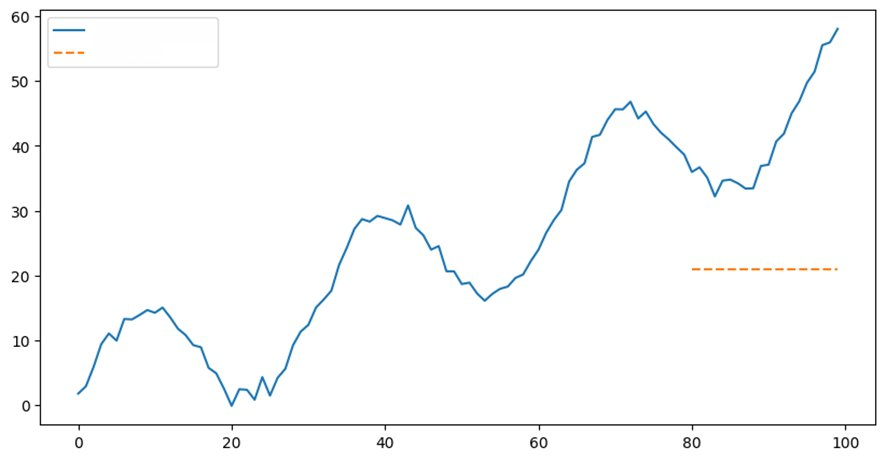
A common mistake in time series forecasting implementation is the inadequate selection of evaluation metrics, which not only distorts the view of model effectiveness but also leads to suboptimal decisions. For example, Hewamalage et al.^[2] criticize the excessive use of mean squared error (MSE) and mean absolute error (MAE) without considering specific data characteristics, such as seasonality and non-stationarity. Figure 1 illustrates this, showing that forecasts based on the mean of the training data can be inadequate. It is observed that the forecast (dashed line) is a constant horizontal line reflecting the mean of the training data. This approach completely ignores the trends and seasonality present in the data. Using metrics like MSE and MAE without considering these characteristics can lead to misleading evaluations. Although these indicators may be suitable in some cases, they fail to capture the complex dynamics of time series, such as trends and seasonality. Poorly chosen evaluation metrics can result in forecasts that appear satisfactory in terms of average error but actually fail to reflect the underlying reality of the temporal data.

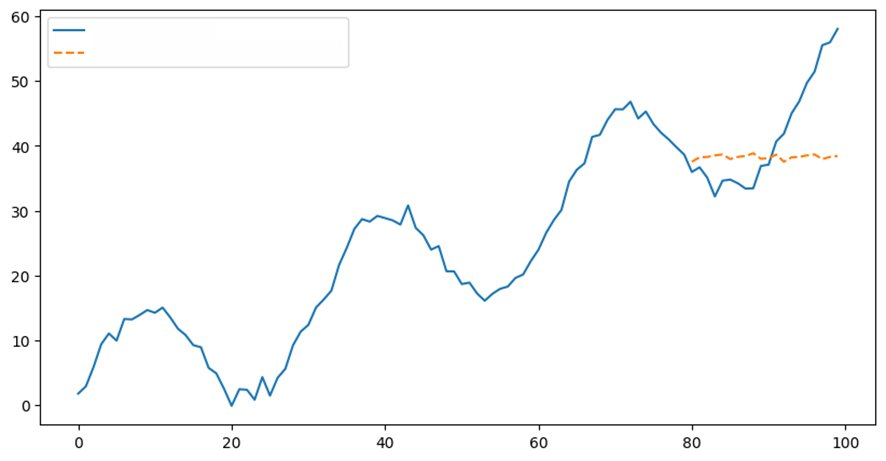
Another common error highlighted in the literature involves the inadequate treatment of time dependence in predictive models. Many analysts do not consider that observations in a time series are correlated, which contradicts the basic assumptions of many traditional statistical methods. As Zemkoho^[3] explained, ignoring autocorrelation between consecutive periods can lead to an underestimation of uncertainty and forecasts that do not reflect the true dynamics of the data. This oversight is particularly important in models such as autoregressive integrated moving average (ARIMA) and exponential smoothing, in which the assumption of independence can invalidate predictions and compromise the integrity of the conclusions obtained. Figure 2 shows that the forecasts generated by the exponential smoothing model (dashed line) fail to capture the trends and seasonality present in the original data. The forecast attempts to capture a moving average of the data, but does not follow the true dynamics of the time series. This results in predictions that do not fully reflect the fluctuations and dynamics of the actual data.

Based on the discussion about the importance of considering time dependence when modeling time series, it is equally important to address another fundamental concept in time series analysis: stationarity. As Zemkoho^[3] emphasized, the assumption that a time series is stationary — meaning its statistical properties, such as mean and variance, do not change over time — is crucial for the application of many statistical models. However, many real-world series exhibit trends or seasonality, which violates this assumption. Failure to test and adjust for non-stationarity can result in a model that appears adequate but actually fails to capture the underlying data dynamics, leading to inaccurate and potentially costly forecasts.

Once non-stationarity is identified through appropriate tests, techniques such as differencing and logarithmic transformations are frequently used to stabilize variance and make the mean constant over time, i.e., these techniques are used to prepare data for models that assume stationarity, such as ARIMA models. However, the choice of the degree of differencing or type of transformation should be carefully adjusted to avoid over-differencing, which can introduce noise and cause the loss of important information from the original signal. Therefore, it is recommended to determine the appropriate number of differences to ensure model adequacy without compromising data integrity through cross-validation and the use of information criteria, such as the Akaike information criterion (AIC).

The implementation of differential and logarithmic transformation techniques is crucial for dealing with the non-stationarity of time series and can be achieved using libraries such as pandas and statsmodels which run in Python. For example, the adfuller() function in the statsmodels.tsa.stattools module allows you to perform augmented Dickey-Fuller (ADF) tests directly on your data while using numpy or pandas libraries to simplify transformations like logarithmic transformations through vector operations. In summary, these tools not only facilitate the work but also help improve the quality of time series analysis.

Interpreting the results of stationarity tests and applying the correct transformations are challenges that require a deep understanding of the technical background and the data. Even when using advanced tools, such as the Python language, it is necessary to be aware of potential pitfalls, such as incorrect interpretation of p-values or unnecessary application of differencing, which can compromise the quality of predictions. To mitigate these risks, an iterative modeling approach is recommended, in which each step is validated using data visualization and fine-tuning of performance metrics, such as AIC. This ensures that the changes actually improve the predictive power of the model without introducing biases or overfitting.

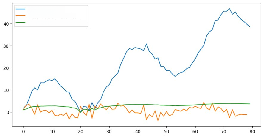
The graph in Figure 3 shows the original time series data (blue line) with trends and seasonality, compared with the differenced (orange line) and logarithmically transformed (green line) data. The ADF test results on the original data indicated that the series was not stationary (ADF statistic of 0.292 and p-value of 0.977). After differencing, the series became stationary (ADF statistic of -6.094 and p-value of 1.02e-07). Transforming the series to stationarity is a necessary step for many time series modeling techniques. However, these transformations must be performed carefully to ensure that the data is adequately prepared for subsequent modeling.

Hewamalage et al.^[2] emphasize that, while these tests are useful, it is also important to understand their limitations and correctly interpret their results. For example, they caution against over-reliance on automated stationarity test results, which may fail to capture important nuances in the data’s temporal structure. In other words, while these tests can provide a useful indication of stationarity, they do not replace a deep understanding and careful analysis of the data.

It is worth noting that the effective implementation of time series models in real-world scenarios requires more than just accurate fitting; it also demands a clear understanding of the context in which the forecasts are applied. In sectors such as finance, retail, and energy, robust models can mean the difference between significant profits and losses. Therefore, in addition to accuracy, models must also be adaptable and sensitive to economic, seasonal, and regulatory changes. Continuous collaboration between data analysts and domain experts is recommended to ensure that forecasts are not only accurate but also relevant and applicable to the strategic decisions they face.

The development of time series modeling techniques has led to significant advances, especially with the integration of machine learning methods. Hybrid approaches that combine traditional statistical techniques with machine learning methods have proven to be particularly effective. For example, ARIMA models can be used to capture linear patterns in data, while neural networks are used to model nonlinear components. This combination can significantly improve forecasting results compared to using a single method^[4].

Recently, the effectiveness of hybrid models was demonstrated in the M4 time series forecasting competition, organized by Spyros Makridakis and the International Institute of Forecasters (IIF). The M4 competition, part of a series of competitions initiated in 1982 by Makridakis, involved forecasting 100,000 time series using 61 different methods, highlighting the importance of this approach ^[5],[6]. Currently, the M4 has been succeeded by the M5, continuing the tradition of evaluating and improving forecasting methods. However, it is important to highlight that the accuracy of these forecasts depends on the appropriate choice of evaluation metrics and the correct implementation of validation techniques, such as cross-validation, for example^[7].

Furthermore, the combination of different network architectures — such as recurrent neural networks (RNN), long short-term memory (LSTM) and convolutional neural networks (CNN) — has shown interesting performance in various applications by capturing complex and non-linear patterns present in the data^[2].

The continuous advancement of emerging technologies, such as machine learning and artificial intelligence, promises not only to increase the accuracy of predictions, but also to automate and optimize data analysis processes at scale. In the future, predictive models are expected to become even more integrated with real-time decision-making systems, providing instant insights and democratizing access to data analysis.

References

[1] Morettin P.A.; Toloi C.M.C. Análise de séries temporais: Modelos lineares univariados. 3ed. São Paulo: Blucher; 2018.

[2] Hewamalage H.; Ackermann K.; Bergmeir C. Forecast evaluation for data scientists: common pitfalls and best practices. Data Mining and Knowledge Discovery. 2023; 37(2): 788-832. https://doi.org/10.1007/s10618-022-00894-5.

[3] Zemkoho A. A basic time series forecasting course with Python. Operations Research Forum. 2023; 4(2): 1-43. https://doi.org/10.1007/s43069-022-00179-z.

[4] Zhang G.P. Time series forecasting using a hybrid ARIMA and neural network model. Neurocomputing. 2003; 50: 159-175. https://doi.org/https://doi.org/10.1016/S0925-2312(01)00702-0.

[5] Smyl S. A hybrid method of exponential smoothing and recurrent neural networks for time series forecasting. International Journal of Forecasting. 2020; 36(1): 75-85. https://doi.org/10.1016/j.ijforecast.2019.03.017.

[6] Makridakis S.; Spiliotis E.; Assimakopoulos V. The M4 Competition: 100,000 time series and 61 forecasting methods. International Journal of Forecasting. 2020; 36(1): 54-74. https://doi.org/10.1016/j.ijforecast.2019.04.014.

[7] Bergmeir C.; Benítez J.M. On the use of cross-validation for time series predictor evaluation. Information Sciences. 2012; 191: 192-213. https://doi.org/10.1016/j.ins.2011.12.028.

How to cite:

Silva J.E. Best practices and common errors in time series modeling. E&S Journal. 2024; 5: e20240028.

About the author

José Erasmo Silva – Advisor Professor MBA Data Science and Analytics – Federal University of Bahia – Postgraduate Program in Accounting – PPGCONT– Avenida Reitor Miguel Calmon, s/n Canela – CEP: 40231-300 – Salvador/BA, Brazil